A Tutorial on the Penetration of Kinetic-Energy (KE) Rounds

Introduction

The design of short KE projectiles has changed drastically with increasing muzzle velocity producing much higher impact velocities on the target. During World War II muzzle velocities were typically lower than 1 000 m/sec. The best penetration could be achieved by very hard non-deforming projectiles, which penetrated and perforated by volume deformations in the target plates or by plugging out a hole, working like a piston. The energy threshold for the projectile can be described by the “volume deformation” as follows:

$0\text{.}5\cdot m\cdot v_j^2=C_v\cdot D^2\cdot d$ (1)

or by plugging as:

$0\text{.}5\cdot m\cdot v_j^2=C_p\cdot D\cdot d^2$ (2)

where m is the projectile mass, v_j the impact velocity, D the projectile diameter, d the target plate thickness (or the line-of-sight thickness d/cosθ for inclined plates, where θ is the NATO angle), and C_v and C_p are the corresponding constants for volume deformation and plugging respectively.

In the Equation (1) the diameter D is raised to the power of two and the plate thickness d to the power of one, whereas in the plugging Equation (2) the projectile diameter D is raised to the power of one and the plate thickness d to the power of two.

In reality the perforation mechanism lies in between the extremes of Equations (1) and (2). In practice the initial penetration by a non-deforming projectile of a thicker target plate is typically by volume deformation and the final perforation is by a more-or-less plugging process. The critical velocities for plate perforations are been described by the Krupp and the DeMarre equations in which the sum of exponents for the projectile diameter D and the plate thickness d is three or approximately three.

The sum of the exponents in the Krupp equation is exactly three:

$E_{\text{cr}}=C_K\cdot D^{1\text{.}\text{67}}\cdot d^{1\text{.}\text{33}}$ (3)

whereas the sum of the exponents in the DeMarre equation is approximately three:

$E_{\text{cr}}=C_M\cdot D^{1\text{.}5}\cdot d^{1\text{.}4}$ (4)

where E_cr is the critical kinetic energy for a perforation and C_K and C_M are the corresponding constants [1].

As muzzle velocities increase the contact pressure begins to exceed the strength of possible projectile materials, requiring the use of very hard materials such as tungsten carbide. The velocity limit between the possibilities of non-deformation projectile penetrations and eroding projectiles is approximately 1 000 m/s.

Current projectile velocities are running in the so-called partially hydrodynamic regime where fluid dynamic behaviour of the materials provides the dominant features. For ordnance velocities in the range of typically 1 400–1 800 m/s, however, the hardness of the projectile is still important.

The development of the projectiles extends from the full-caliber projectiles, to the so-called APDS (Armour Piercing Discarding Sabot, spin-stabilised) projectiles, to APDSFS (Armour Piercing Discarding Sabot Fin Stabilized) projectiles. The penetrators are reduced in diameter and elongated in length. They are accelerated and launched from the gun tubes with the help of the sabots. The projectiles are typically made from heavy metals, like sintered tungsten alloys or depleted uranium.

Early KE projectiles were only spin-stabilized. But this can be done only over a length-to-diameter ratio of about 3.5. To meet the desired increase in lengths, the long rods have to be fin-stabilized and are now fired from smooth-bore guns or from rifled guns using slipping driving bands. While there had initially been doubts about the hit probability of long-rod projectiles fired from smooth-bore guns, they can now achieve the same hit dispersion on the target as those fired from rifled guns.

These projectiles, with their very low area-to-mass ratio, undergo a very low reduction in velocity as the move through the air—typically 30–50 m/sec over a distance of 1 000m—and therefore have short flying times over extremely long distances. They also have high impact velocities and good hit probabilities against moving targets.

Penetrations of APDSFS projectiles

Rule of thumb

For these long heavy metal projectiles with high velocities, we can use following equation derived from the modified Bernoulli equation:

$P\equiv L\cdot \sqrt{{\rho }_P/{\rho }_t}$ (5)

where P is the penetration in the target, L is the effective projectile length and ρ_P and ρ_t are the projectile and target densities. This simple equation neglects, besides other parameters, any projectile strengths and does not take velocity into account. In the typical ordnance velocity range of 1 400 m/sec to 1 800 m/sec, projectiles do not penetrate as far as this equation predicts. However, velocity can be accounted for by the inclusion of an efficiency factor η in Equation (5):

$P=\eta \cdot L\cdot \sqrt{{\rho }_P/{\rho }_t}$ (6)

For an impact velocity of 1 700 m/s the efficiency factor η is about 2/3. For heavy metal projectiles against steel targets, the square root factor is approximately 3/2, so that Equation (6) simplifies to:

$P=L$ (7)

Equation (7) therefore provides a very rough rule of thumb for the penetration capability of long-rod projectiles of sintered-tungsten alloys or depleted uranium in the higher ordnance velocity range. Let us look at a numerical example. Modern heavy-metal projectiles of 600-mm effective length have a penetration/perforation capability of about 600 mm. This is a realistic value for such fin-stabilized long-rod penetrators, made from depleted uranium (DU) or tungsten-sintered alloys, with densities of about 18 g/cm³.

$P=2/3\cdot \text{600}\text{mm}\cdot \sqrt{\text{18/7}\text{.}8}=\text{600}\text{mm}$ (8)

The key to the design of more-efficient penetrators with greater penetration is to elongate their lengths (L). To avoid bending of the now thinner rods, a number of sophisticated KE penetrator ideas—such as the so-called jacketed rods or telescope designs—are under investigation.

Although some investigator focus on achieving high length-to-diameter ratios or large L/D values, I prefer to emphasise only the length L to give more penetration. A high L/D ratio can be achieved by a projectile with a relatively small diameter which can therefore be disturbed much more easily by special moving armours—like explosive reactive armour or bulging armour—compared to penetrators with thicker diameters, but shorter lengths.

Hohler and Stilp diagram

Hohler and Stilp [2] published a paper with a large number of tests with cylindrical projectiles of different L/D ratio, and of steel and tungsten sintered alloys from low velocity up to 4 000 m/s by using a light gas gun. In agreement with Hohler the author has produced from the different data the simplified diagram of Figure 1.

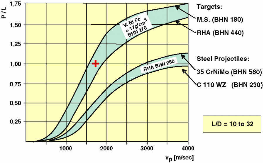
Figure 1 shows the ratio P/L of the penetration P to the projectile lengths L as a function of the projectile impact velocities v_P for long rod penetrators of the L/D ratio of 10 to 32. Although model-scaled projectiles at the diameters of 4–6 mm were used to obtain the results in Figure 1, these data correlate well with results from full-scale projectiles.

The rod projectiles of heavy metal with density of around 17 g/cm³ (tungsten-nickel-iron sintered alloy) and strength of BHN 270 are fired against mild steel (BHN 180) and armour-steel (RHA–BHN 440) targets. These curves show that heavy metal projectiles achieve the scaled penetration P/L of “one” against mild steel at a velocity of 1 600 m/s, but achieve only 0.75 against high-grade armour steel. To obtain the P/L value of “one” for high-hardness armour steel (BHN 440), a velocity of 1 800 m/s to 1 900 m/s is necessary. But as marked by the cross on Figure 1, the P/L value of “one” against medium-hardness steel is achieved with 1 700 m/sec. This confirms the rule-of-thumb described in the previous section.

The steel rods are fired against a medium-hardness armour steel targets (BHN 280). However, the projectiles have now different strengths, soft iron (C110 WZ/BHN230) and high hardness chromium-nickel-molybdenum steel (Cr/Ni/Mo—BHN 580). It can be seen the steel projectiles with the higher hardness achieve more penetration in the target compared to the softer steel projectiles.

Figure 1 demonstrates that neither the strength of the target nor the strength of the projectile can be fully neglected in the penetration behaviour of long-rod penetrators. They are, however, a magnitude less important than the length and the velocity, especially in the modern ordnance velocity range of 1 400 m/s to 1 800 m/s.

Lanz/Odermatt/Jeanquartier equations

Perforation

In 1992 Lanz and Odermatt [3] presented a new equation for KE-round penetration, which included both velocity and target strengths. After more firings, with different projectile lengths ranging now from 90 mm to 825 mm, and projectile diameters from 8 mm to 32 mm, the constants for their first equation were modified slightly and presented in 1995 in a paper by Jeanquartier and Odermatt [4]. These very useful equations for designing and predicting KE-round performance are presented here in detail. Their available parameters are illustrated in Table 1. A practical numerical example is also presented.

Penetrator Properties

Length L 90–825 mm

Diameter D 8–32 mm

Length-to-diameter ratio L/D 11–31

Rod density ρ_P 17 000–17 750 kg.m³

Rod mass m_P 0.1–9 kg

Impact velocity v_P 1 100–1 900 m/s

Target properties

Plate thickness d 40–400 mm

Tensile strengths R_m 800–1 600 MPa

Obliquity (NATO angle) θ 0-74°

Density ρ_t 7 850 kg/m³

Figure 2 illustrates the various parameters. It should be emphasized that the geometric length L_eff of the projectiles can be measured and the “effective length”, L_W has to be used in the equations. If the projectile has a conical tip then a cylinder with the same radius as the following projectile part with the same mass has to be calculated. But for the end region, the length has to be reduced always by one diameter of the cylindrical end section, as shown in Figure 2. In contrast to the above original publications, L_W has to be always used for the “effective projectile lengths” compared to the geometric L_eff. This shortening by one D has to be taken into account in all of the following equations. As diameter D has to be measured at the back of the threat.

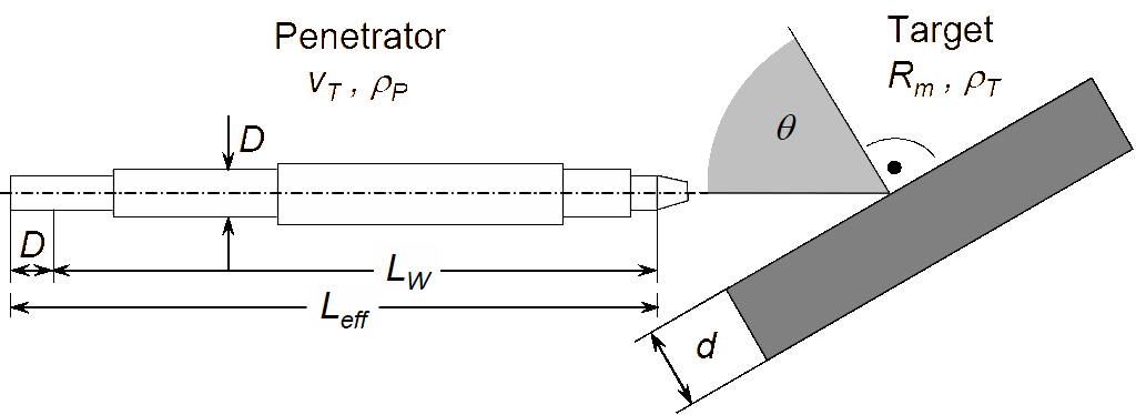
The following equation; which is principally an empirical modification of Equation (5), gives the limit of the perforation of APDSFS-projectiles on the basis of 74 test results with 19 different parameters. The penetration scaled down by the diameter L_W is given as follows:

$P/L_W\equiv f\left(\lambda \right)\cdot (\text{cos}\theta {)}^{-m}\cdot \sqrt{{\rho }_P/{\rho }_t}\cdot e^{-c\cdot R_m/({\rho }_P\cdot v_P^2)}$ (9)

where:

P perforation length

D diameter of the projectile (at the back of the threat)

L_eff projectile along the heavy metal length (see Figure 2)

L_W effective projectile length (L_W=L_eff–D) (for the conical tip has to be used a cylinder of diameter D with equal mass)

λ _eff L_eff /D

λ L_W /D

θ NATO angle of an inclined plate to the velocity vector of the projectile

m exponent for plate inclination

ρ_P density of projectile (kg/m³)

ρ_t density of target (kg/m³)

R_m target strengths in Pa

c correction factor for target strengths-see Equation (12)

v_P projectile impact velocity (km/sec)

If the function of L_W/D is less than 20, it must be corrected. The equation is given by:

$f\left(\lambda \right)=1+3\text{.}\text{94}\cdot \left\{1-\text{tanh}\left[\right(L_w/D-\text{10})/\text{11}\text{.}2]\right\}$ (10)

The hyperbolic tangent is defined as:

$\text{tanh}\left(x\right)=(e^x-e^{-x})/(e^x+e^{-x})$ (11)

The constants for the above equation are found by fitting the experimental achieved results, as presented in Figure 3.

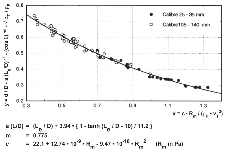
For the constant c, Jeanquartier/Odermatt [4] have presented the following equation:

$c=\text{22}\text{.}1+\text{12}\text{.}\text{74}\cdot {\text{10}}^{-9}\cdot R_m-9\text{.}\text{47}\cdot {\text{10}}^{-\text{18}}\cdot R_m^2$ (12)

where R_m is in Pa.

The constants for the c Equation (12) are found by fitting the experimental results as shown in Figure 4.

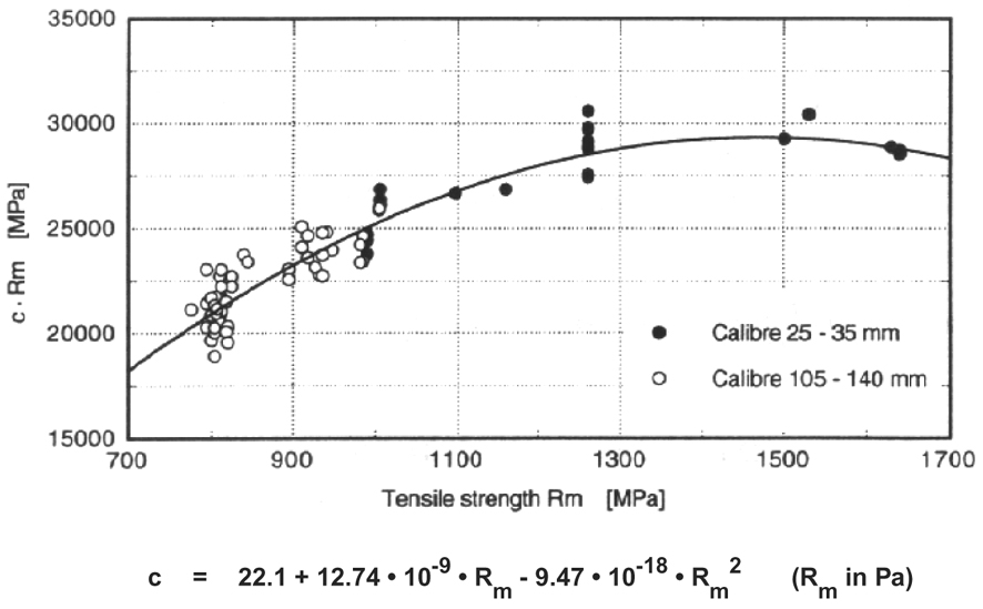
A numerical example for this equation should be given in the following:

L_eff = 400 mm projectile length

D = 25 mm projectile diameter

λ_eff = 16 (400 mm / 25 mm)

L_W =(L_eff – D) = 400 mm – 25 mm = 375 mm

λ =L_W/D = 15

θ = 60° NATO angle of the target plate

ρ_P = 1 7500 kg/m³ projectile density

ρ_t = 7850 kg/m³ target density

R_m = 1.000 N/mm² target strength (=10⁹ Pa)

v_p = 1.800 m/s projectile impact velocity

Placing these values into the Equation (13) gives:

$P/\text{375}=f\left(\lambda \right)\cdot (\text{c}\text{o}\text{s}\text{60}°{)}^{-0\text{.}\text{225}}\cdot \sqrt{\text{17500}/\text{7850}}\cdot e^{-c\cdot {\text{10}}^9/(\text{17500}\cdot {\text{1800}}^2)}$ (13)

$f\left(\lambda \right)=1+3\text{.}\text{94}/\text{15}\left\{1-\text{tanh}(\lambda -\text{10})/\text{11}\text{.}2\right\}=1\text{.}\text{11}$ (14)

This “short” projectile has about 11% more perforation due to residual penetration effects.

The cosine expression gives also increased penetration for more inclined plates. For the 60° NATO angle about 17% more penetration will be achieved.

$(\text{cos}\text{60}°{)}^{-0\text{.}\text{225}}=1\text{.}\text{169}$ (15)

The density ratio gives with the square root law about 50% more penetration compared to steel projectile.

$\sqrt{\text{17500}/\text{7850}}=1\text{.}\text{493}$ (16)

The target strength constant c is calculated in the following way:

$c=\text{22}\text{.}1+\text{12}\text{.}\text{74}\cdot {\text{10}}^{-9}\cdot {\text{10}}^9-9\text{.}\text{47}\cdot {\text{10}}^{-\text{18}}\cdot {\text{10}}^{9^2}c=\text{22}\text{.}1+\text{12}\text{.}\text{74}-9\text{.}\text{47}=\text{25}\text{.}\text{37}$ (17)

Finally the exponent value E can now be calculated as follows:

$E=e^{-c\cdot {\text{10}}^9/(\text{17500}\cdot {\text{1800}}^2)}=0\text{.}\text{639}$ (18)

The penetration P path for a 60° inclined target plate is:

$P=\text{375}\cdot 1\text{.}\text{11}\cdot 1\text{.}\text{169}\cdot 1\text{.}\text{493}\cdot 0\text{.}\text{639}P=\text{464}\text{m}\text{m}$ (19)

If a perpendicular target plate arrangement had been used, Equation (13) would calculate a limit value of 397 mm. This is exactly the value estimated by the rule of thumb for a 400-mm long projectile. But in this case we also have an upper limit of velocity and a medium-hardness RHA target. So this value is very reasonable.

Residual velocities

Jeanquartier/Odermatt [4] also measured the residual velocities of the projectiles after they had perforated the targets. They found the following equation for long-rod penetrators:

$v_R/v_P=1+a\cdot \text{ln}(1-d/d_{\text{lim}})$ (20)

As illustrated in Figure 5, Equation (20) can be fitted closely to the experimental data if a value of a=0.14 is used.

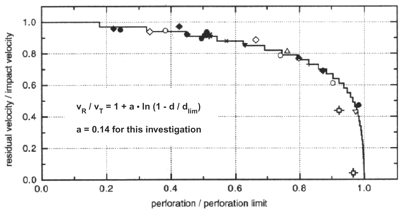
For our numerical example of a 300-mm perpendicular steel plate, where the limit thickness was calculated to be 397 mm, Equation (20) can be written:

$v_R/v_P=1+0\text{.}\text{14}\cdot \text{ln}(1-\text{300}/\text{397})=0\text{.}\text{803}$ (21)

With the impact velocity of 1 800 m/s, the residual velocity is:

$v_R=0\text{.}\text{803}\cdot \text{1800}\text{m/s}=\text{1445 m/s}$ (22)

Residual projectile length

Jeanquatier/Odermatt [4] also provide an equation for the effective residual projectile length whereby, as illustrated in Figure 6, the effective length is the sum from broken rod pieces.

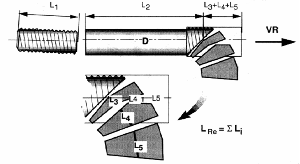
The residual lengths after the original effective lengths L_e is given by the following equation:

$L_{\text{Re}}/L_e=1-(1-b)\cdot d/d_{l_{\text{im}}}-b\cdot (d/d_{\text{lim}}{)}^2$ (23)

The coefficient b is a function of the projectile impact velocity. In the range of 1 400 m/s to 1 500 m/s, b=0.2. At higher velocities the b=0. That means that the parabolic curve is a straight line in Figure 7. If the velocities are smaller than 1 400 m/s, the b value will be larger than 0.2 and the parabolic curve has a smaller radius.

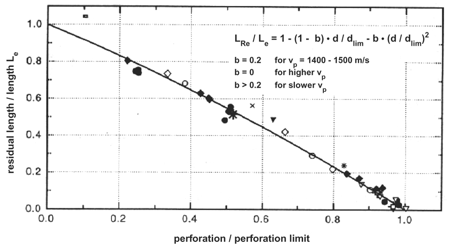
The residual lengths were measured from a flash X-ray picture taken relatively close to the perforated plate. In larger distances (further than 0.5m, for example) the pieces were more dispersed and were also tumbling.

In our numerical example the velocity is 1 800 m/s; then b=0. This means the residual length of the projectile is proportional to d/d_lim. For d = 300 mm and d_lim = 397 mm the residual length L_Re is therefore given by:

$L_{\text{Re}}/L_e=1-\text{300}/\text{397}=1-0\text{.}\text{756}=0\text{.}\text{244}$ (24)

With the effective lengths L_e of 400 mm for this example the effective residual lengths L_Re will be 400 × 0.244 = 98 mm. Again, Jeanquatier and Odermatt [4] have shown this equation to have a relatively good experimental basis.

Summary

As a rule-of-thumb, the perforation capabilities of heavy metal long-rod penetrators can be very simply predicted by their length. Their velocity dependence can be better seen by the Hohler/Stilp diagram or can be calculated by the Lanz/Jeanquartier/Odermatt equation, which takes also into account the target strength.

These Lanz/Jeanquartier/Odermatt equations are also very helpful in layout and design studies for the improvement of the penetrators and for vulnerability predictions with parameter variations of the performance of modern APDSFS projectiles.

References

Author

Prof. Dr. M. Held is with TDW/EADS, Schrobenhausen, Germany He is experienced in warhead design, blast, shaped charges, EFP´s and fragments. Through his world-wide teaching in armour concepts and warhead layouts he also describes the threat by kinetic energy rounds or KE projectiles. Tel: 49-8252-996-345, Fax: .49-8252-996-126, E-mail: Manfred.Held.@TDW.LFK.EADS.net.

References

[1] M. Held, State-of-the-art in Heavy Armour Principles, Lecturing Notes, IAT Austin Texas, USA, May 1999, or, M. Held, Survivability of Armoured Vehicles, Lecturing Notes, Cranfield University, UK, March 2002.
[2] V. Hohler and A. J. Stilp, “Penetration of Steel and High Density Rods in Semi-Infinite Steel Targets”, 3<sup>rd</sup> International Symposium on Ballistics, Karlsruhe, Germany, H3:1-12, 1977.
[3] W. Lanz and W. Odermatt, “Penetration Limits of Conventional Large Caliber Anti Tank Mines / Kinetic Energy Projectiles”, 13<sup>th</sup> International Symposium on Ballistics, Stockholm, Sweden, Vol. 3, pp. 225–233, 1992.
[4] R. Jeanquartier and W. Odermatt, “Post-perforation Length and Velocity of KE Projectiles with Single Oblique Targets”, 15<sup>th</sup> International Symposium on Ballistics, Jerusalem, Israel, Vol. 1, TB 32, pp. 245–252, 1995.