
Volume 6, Number 3, November 2003
Combat Entropy as a Measure of Effectiveness
- 1 Land Operations Division, DSTO Edinburgh, PO Box 1500, Edinburgh, Australia, 5111.
Abstract
This study investigates the use of casualty based entropy and the entropic phase space developed by Carvalho-Rodrigues et al, to determine its usefulness as a measure of effectiveness without further investigation into the theoretical meaning of the method. The change in combat entropy (ΔS) method for time-independent data of Carvalho-Rodrigues et al was tested using historical analysis. We then extended the ΔS method and showed its utility for time-dependent data—where Carvalho-Rodrigues et al applied an entropic phase space (EPS). While the entropic phase space was determined to be a poor outcome predictor we found that the ΔS between two forces is a good predictor of attrition based warfare outcomes with a successful force usually one that can maintain lower entropy for a greater time period.
Introduction
In the early 1990’s, Carvalho-Rodrigues et al [1,2] explored the use of an entropy concept to measure unit performance. They developed a casualty-based entropy (combat entropy) measure and an entropic phase space (EPS) to “predict” attrition-based combat outcomes. This study investigates and reviews the application of casualty-based entropy and the EPS in order to determine its utility without investigating further the theoretical meaning of the method. This was achieved by analysing historical and independent simulation data for the entropy method and comparing with a Lanchester model—and where necessary clarifying and amending elements of the entropy measure. Amendments were made for the EPS where the previous model was abandoned and the change in combat entropy extended to cover time-dependent data as well as time-independent data.
Attrition-based models
Lanchester model
Traditionally, the Lanchester models [3,4,5] are a set of differential equations that have been employed to predict combat outcomes. They are based on the assumption that the attrition suffered by either side in battle is a function of the numerical strengths of the forces involved and the efficiency of their respective weapons. For example, the direct fire form (Equation (1)) gives the rate of casualty production for a side, where A and B are the number of each sides’ surviving combatants at time, a and b are the casualty rates for which B can kill A and A can kill B, respectively.
dA/dt = -aB and dB/dt = -bA (1)
These equations may be solved with respect to time to give the number of surviving units on each side, respectively, after the start of battle. As a result, battle outcome predictions can be made.
Carvalho-rodrigues combat entropy
Combat has been accepted as a dissipative phenomenon [1,6] (and this is particularly the case in attrition-based warfare) and Carvalho-Rodrigues [1] was able to link the derivation of ’s information theory form of entropy for combat with the form for thermodynamic entropy, which they
propose is a more suitable way of representing combat in these circumstances. Irrespective of the area of application, entropy is defined as S = –p ln p [7,8], where p represents the probability of the state of a system. For example, gas molecules trapped in a bottle will have an amount of disorder associated with them, described by a probability, p (as a result of collisions with other molecules). To draw a simple analogy for a military situation, replace the gases with soldiers in combat and make the bottle a battlefield. The probability is now the state of disorder of those soldiers (or the probability of a casualty occurring). Carvalho-Rodrigues [1] developed Equation (2) as the form of casualty-based entropy (coined combat entropy) by representing the p as casualty proportions of a total force size—being the probability of each casualty (note [1,2] used H instead of S to represent entropy).
(2)
where ci = casualties at time t;
N = force size (and Ni = N – ci at t); and
i = red or blue.
Carvalho-Rodrigues et al use the form ΔS= Sdefence–Sattack as a predictive tool for combat outcomes. At some time, t, in a battle (for time-dependent data or at the end of a battle for time-independent data) S was calculated to determine which side was likely to win, accounting for reinforcements, in that battle. They used this ΔS for time-independent data and an EPS for time-dependent data outcome predictions.
Like the Lanchester model, this entropy model was purely attrition-based but the principle of the measure is different. Carvalho-Rodrigues et al found that it was unlikely that their results for ΔS (only used on time-independent data) were produced at random. Firstly, the entropy model provided a good prediction method which gave significant results.
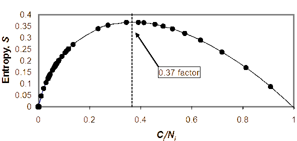
A significant result of the Carvalho-Rodrigues et al [1,2] work was that S had a maximum for ci/Ni = 0.37 (or 37% casualties). An example for the Les Mans battle data is shown in Figure 1 with the 0.37 factor marked. This result was more than just an empirical consistency of the data used in Equation (2) (and of military findings), but a mathematical consequence of the function used (that is, Smax = e when ci/Ni = 1/e = 0.37). We support this finding of Carvalho-Rodrigues [1] which shows a correlation between the empirical findings from the data (and anecdotes) and the mathematical consequence of the entropy function. It implies that in terms of the combat entropy of a military force, once a casualty rate has surpassed 37%, the force enters a negative feedback cycle with an ever-increasing rate of casualties. Such a factor might imply a point exists at which a force loses its ability to work as an effective unit. Indeed, this factor has been identified [2,9,10] as a point where, when losses exceed 37%, most battles will usually break off or result in loss for that side.
Carvalho-Rodrigues et al performed analyses of time-dependent historical data and developed what they termed the EPS. This EPS is a two-dimensional plot of the (entropy of the defender (Sd)/0.37) versus the (entropy of the attacker (Sa)/0.37). This “phase space” was then split into four quadrants and the shape of the plot through the quadrants was said to be a predictor of combat outcomes for time-dependent data. Figure 2 shows an outline of an EPS plot. Carvalho-Rodrigues et al in [2] deduced from their data that the risk of taking the initiative and higher risks and enduring higher casualties (the rate of which will slow) initially, will pay off as the opposition then climbs in entropy and cannot reverse the process as has already happened for the risk taker. This results in the “arrows of time” of Figure 2 which seem contrary to what would be expected.
![The EPS and “arrows of time”. [2]](/journals/journal-of-battlefield-technology/volume-06/issue-03/assets/6-3-7-dexter/figures/figure02.gif)
Validity of combat entropy and the entropic phase space
Historical data
To investigate the combat entropy and then understand the EPS this study analysed as much data as could be obtained from [1,2] as well as data from other battles (both real and simulated—independent simulation data was originally included as a result of the unpromising nature of the historical battle data outcomes for EPS analysis) that was accessible in sufficient detail [2,4,5,9-12]. The independently run simulation data was sourced from both (small unit) and JANUS (campaign level) military wargames from other studies. The utility of the simulation data was to provide an expanded data set for the time-dependent analyses and to provide “Lanchester” type results for further comparison for the time-independent data. As shown in the Annex to this paper, data was taken for historical battles going back to the 17th century. As tactics have significantly changed over that period, it provides an opportunity both to determine the relative success of the ΔS method, EPS and basic Lanchester, and to identify how generally these can be applied.
Carvalho-Rodrigues et al [2] placed size of battle and manoeuvre constraints on their data sets only testing the model against a small subset of battle data. This study has not stayed within these constraints, due to limited data. The inclusion of battles with manoeuvre has also allowed a preliminary test of robustness of the change in combatentropy model.
Time-independent data
A list of time-independent battle data, with corresponding winner predicted by ΔS, winner as predicted by a Lanchester attrition model, both as calculated by the author, and the actual winner as stated historically is given in the Annex.
Table 1 shows and compares the correct and incorrect predictions for time-independent data used to calculate ΔS and the Lanchester predictions, as well as the percentage predicted correctly and corresponding χ2 [13] values. It also shows the time-dependent results for the ΔS, Lanchester and EPS predictions for comparison and which are discussed below.
In order for direct comparison with the results of Carvalho-Rodrigues et al the resultant χ2 values were tested against a null hypothesis that these values could have been generated at random. The results for both the Lanchester and ΔS model predicted better than the Lanchester model, showing the potential of the entropy method to be used to describe combat (as attrition based conventional warfare) better than more traditional methods.
The reason some battles were predicted incorrectly can be explained by the nature of those battles. Further investigation of some battles showed they cannot be modelled so generically and suggest that they contain particular non attrition factors. Some battles involved a side that had suffered heavy attrition (as percentages of the force), or which were overwhelmingly outnumbered, but which endured to obtain a successful outcome. For example the battle for Iwo Jima in 1945 between the US and Japan saw a tiny island overpopulated with soldiers for the battle duration where the Japanese were dug in and could fire upon the whole island from their positions and rarely came above ground to fight. The marines were confronted with entrenched troops and had to adapt to use new tactics for fighting the Japanese in order to succeed.
| Correct Prediction | Incorrect Prediction | % Correct | χ2 Significance Level | |
|---|---|---|---|---|
| Time-independent | ||||
| ΔS | 91 | 14 | 87 | >99.9% |
| Lanchester | 70 | 35 | 67 | ~99% |
| Time-dependent | ||||
| ΔS | 19 | 1 | 95 | >99.9% |
| EPS | 6 | 14 | 30 | <90% |
| Lanchester | 19 | 1 | 95 | >99.9% |
In another example, the battle for in the Yom Kippur War of 1973, started with deception and surprise and a pre-emptive strike from the Arab attackers and resulted in a very high intensity conflict with the defending side required to adapt very quickly with the changing situation. In the 1966 Battle of Long Tan, the Australian Troops who were outnumbered and boxed in adapted to fight in order to survive and succeed, which they did against a much larger force. In each of these cases, the attrition values were not the primary determinants of the battle outcomes, hence any attrition measure would not be appropriate.
Time-dependent data
In their research Carvalho-Rodrigues et al [1,2] scoped the behaviour of the entropy of a force over time and predicted some trends that should be evident. Figure 3 shows the trends for a force (as determined by Carvalho-Rodrigues et al), which should be evident if a force is to succeed or be defeated. In this they show that a successful force will show some increase in “entropy” but will then decrease, and that a force being defeated will undergo a steady increase in the entropy, which never decreases.
![Entropy trends for battle success according to Carvalho-Rodrigues et al [2].](/journals/journal-of-battlefield-technology/volume-06/issue-03/assets/6-3-7-dexter/figures/figure03.gif)
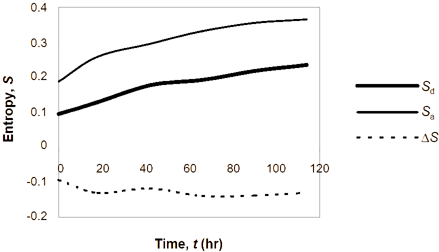
For the data analysed for this study, the trends predicted in Figure 3 were rarely observed in the time-dependent data. For example Figure 4 shows entropy over time for the Westwall (1940) and Le Mans-Metz (1944) Battles. The first for Westwall shows the clear trends for both sides that would according to Figure 3, indicate trends for defeat (or stalemate). However, historically, the Sd (US) side was successful. Carvalho-Rodrigues et al used these entropy trends as combat outcome predictors for time-dependent data. We found that these trends were not useful in the prediction of combat outcomes showing correct trends less than 30% of the time.
(a)
(b)
Carvalho-Rodrigues et al [2] used the ΔS as an initial predictor of combat outcomes—for time-independent data. However, this was the only place they utilised this form of combat entropy. We propose and show that for time-dependent data this is also a good predictor. This would imply then that a successful force would be the one which maintains a lower entropy for a greater time period in a plot of entropy (S) versus time. So a plot of ΔS between two sides should show which side is likely to be successful. This would also allow consistency between analyses for both time-dependent and time-independent data.
Figure 4 shows two battles, which were chosen for their very different battle characteristics as examples of the utility of the ΔS method for time-dependent data. In this figure the ΔS line for the Westwall battle is negative the whole time implying the defence has an overall lower entropy which would give the defence () as securing a victory. The second plot for the Le Mans Battle in 1944 is not clear at all and the Sa (GER) side was eventually successful here. In this plot, from the ΔS line it shows for the first 15 days, that the defence have a lower entropy but only just and that it had the advantage there. However, after day 15 the ΔS increases to positive quite significantly, implying that the attacking side from here on should in fact secure a victory due to their overall lower entropy.
The negative entropy achieved in this plot results when the total number of forces for that side (GER) is greater than the initial force size amount due to the arrival of reinforcements. Both plots do show though, that the side able to achieve and then maintain the lower entropy, in these attrition based battles, was eventually the victor. They also show how one side can quickly change the course of a battle for example in the case of the Le Mans-Metz battle, by the Germans providing sufficient reinforcements to prevent the from countering further.
We have found that the shape of the curve is not as important (or as reliable) as the difference between the entropy curves of the two forces (the change in the combat entropy, ΔS). Subsequent analyses by the author showed that the force that is able to maintain the lower “combat entropy” appears to be the victor in most circumstances (that is, maintaining their entropy on the left-hand side of Figure 1).
Table 2 shows the results for the ΔS and Lanchester methods as well as EPS predicted outcomes as calculated by the author and lists actual battle outcomes as stated historically. The summary for these calculations is listed in Table 1 for comparison with the time-independent data. These results show the ΔS and Lanchester methods to be significantly better than the EPS method. In fact, the χ2 values and comparisons with the other time-dependent methods (as well as the overall time-independent results) suggest that the implementation of the EPS is flawed.
| Predicted ΔS | Predicted Lanchester | Predicted EPS | Actual | |
|---|---|---|---|---|
| Historical | ||||
| 1916 | D | A | A | D |
| Westwall 1940 | A | A | A | A |
| —Corps Level 1940 | A | A | D | A |
| —Div Level 1940 | A | A | D | A |
| Le Mans-Metz—Corps Level 1944 | A | A | D | A |
| Le Mans-Metz—Div Level 1944 | A | A | D | A |
| 1945 | D | A | ambiguous | A |
| Independent Simulations | ||||
| Sim E1 | A | A | D | A |
| Sim E2 | A | A | D | A |
| Sim E3 | A | A | A | A |
| Sim E4 | A | A | D | A |
| Sim E5 | A | A | A | A |
| Sim P1 | D | D | A | D |
| Sim P2 | D | D | ambiguous | D |
| Sim P3 | D | D | ambiguous | D |
| Sim P4 | A | A | ambiguous | A |
| Sim P5 | A | A | ambiguous | A |
| Sim H1 | D | D | A | D |
| Sim H2 | D | D | A | D |
| Sim H3 | D | D | A | D |
Our analyses showed that extreme battle results in an EPS plot can become impossible to interpret. An example of this is the Iwo Jima Battle shown in Figure 5 and from Table 2 we see that it is the only occurrence where the ΔS (time-dependent) method failed. This might indicate that the model fails only in extreme circumstances, though only detailed time-dependent analyses would show this to be true.
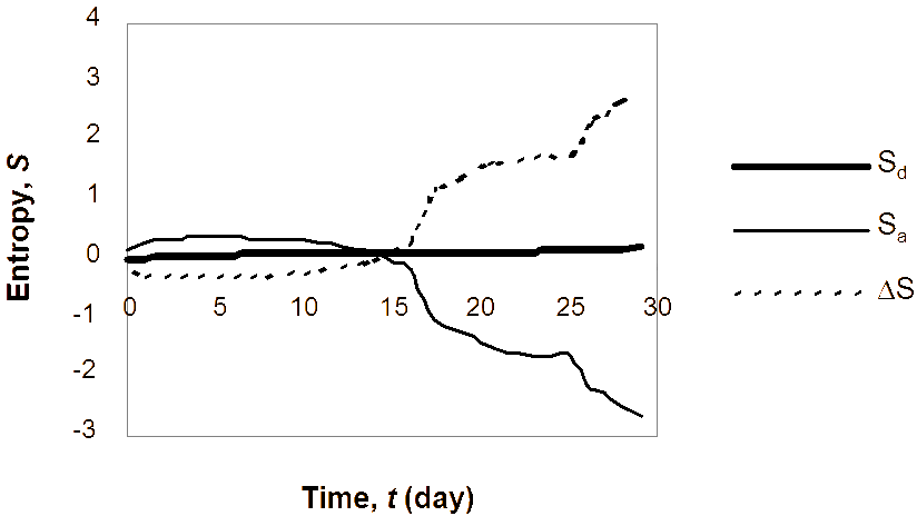
Even though a very small sample set of data was utilised, the conclusion, on the use of the EPS as a predictor of combat outcomes, is that it is unreliable and not clear, whereas the time-dependent ΔS is quite successful when applied to the same battles.
Summary of historical data and model predictions
Over the last 400 years, significant changes have been made to the tactics used in warfare. Table 3 shows that when assessed against this historical battle data (summarised from the Annex), the ΔS method of assessing combat outcomes predicts better than the Lanchester method, for attrition based combat, suggesting that it may provide a better alternative for these analyses. Importantly, the ΔS method still predicts more consistently than the Lanchester method for Post World War II attrition combat showing its relevance and utility in the current age of tactics.
| Tactical Period | ΔS Accurate Predictions | Lanchester Accurate Predictions |
|---|---|---|
| Pre US War of (1674-1759) | 88% | 63% |
| US War of | 38% | 25% |
| Napoleonic Era | 100% | 60% |
| 19th Century Non European Wars | 92% | 42% |
| World War I | 96% | 76% |
| World War II | 80% | 80% |
| Post World War II - today | 86% | 50% |
Conclusions
There are several clear conclusions that can be drawn from this initial study into the utility of combat entropy as proposed by Carvalho-Rodrigues et al [1,2].
This study has shown that the ΔS (change in combat entropy) method is a good predictor of combat outcomes based on attrition values alone for time-independent data. The extension to a wider type of data reinforces the work of Carvalho-Rodrigues et al and shows some robustness to the model.
One of the most important conclusions is that the EPS is not a good outcome predictor. It is recommended that this EPS not be implemented as an analysis method in other areas as it appears to be fundamentally flawed. However, we have extended the time-independent ΔS method to time-dependent data and shown its success in this area further adding to the simplicity and utility of the ΔS method.
Finally, we have shown that although tactics have changed over the last 400 years, and where attrition is the primary determinant of battle outcomes, the ΔS method for attrition scenarios is consistently better than the Lanchester model. Importantly, we have shown that the ΔS method predicts better and more consistently than the Lanchester method for Post World War II attrition, showing its utility and relevance in the current age of tactics.
This shows the entropy method as an alternative analysis tool.
Acknowledgements
Thanks to Drs Neville Curtis and Peter Dortmans.
| Date | Predicted ΔS | Predicted Lanchester | Actual | |
|---|---|---|---|---|
| France/Austria | ||||
| Sinsheim | 1674 | A | A | A |
| Sweden/Brandenburg | ||||
| Fehrbellin | 1675 | A | D | A |
| Late 17th Century | ||||
| 1685 | D | A | D | |
| Killiecrankie | 1689 | D | D | A |
| Jacobite Rebellion | ||||
| Prestonpans | 1745 | A | A | A |
| Culloden | 1746 | D | D | D |
| Britain/France in | ||||
| 1759 | D | D | D | |
| 1759 | D | D | D | |
| American War of | ||||
| 1775 | D | D | A | |
| 1776 | A | A | A | |
| 1777 | A | A | A | |
| 1780 | A | D | A | |
| Cowpens | 1781 | A | A | D |
| Courthouse | 1781 | D | D | A |
| Hobkirk’s Hill | 1781 | D or draw | D | A |
| Eutaw Springs | 1781 | A | A | D |
| Napoleonic Wars | ||||
| 1805 | D | A | D | |
| War of 1812 | ||||
| The | 1813 | A | A | A |
| Chippewa | 1814 | D | D | D |
| Lundy’s Lane | 1814 | D | D | D |
| 1814 | D | A | D | |
| Ecuador/Spain | ||||
| Pichincha | 1822 | D | A or draw | D |
| Revolution | ||||
| 1836 | A | D | A | |
| US/Mexican War | ||||
| 1846 | A | D | A | |
| Resaca de la Palma | 1846 | A | D | A |
| Contreras | 1847 | A | A | A |
| American Civil War | ||||
| 1861 | D | D | A | |
| 1862 | A | A | A | |
| 1862 | D | D | D | |
| 1862 | D | A | D | |
| I | 1862 | D | A | D |
| Kernstown | 1862 | D | D | D |
| 1st Boer War | ||||
| Majuba Hill | 1881 | A | A | A |
| World War 1 | ||||
| 1916 | D | A | D | |
| Somme-Peronne | 1918 | A | A | A |
| Somme-Montdidier | 1918 | A | A | A |
| Yvonne & Odette Positions | 1918 | A | A | A |
| 1918 | A | A | A | |
| Hill 142 | 1918 | A | A | A |
| West Wood I | 1918 | D | A | D |
| West Wood II | 1918 | A | A | A |
| North Wood I | 1918 | A | D | A |
| Bouresches II | 1918 | Draw or A | A | D |
| North Wood II | 1918 | D | A | D |
| North Wood III | 1918 | D | D | D |
| La Roche Wood East | 1918 | A | D | A |
| Amand Farm | 1918 | A | A | A |
| Beaurepaire farm | 1918 | A | A | A |
| Chaudun | 1918 | A | A | A |
| Berzy Le Sec | 1918 | A | A | A |
| Medeah Farm | 1918 | A | A | A |
| Blanc Mont Ridge | 1918 | A | A | A |
| Sommepy Wood | 1918 | A | A | A |
| Ferme Des Granges-Fleville | 1918 | A | A | A |
| Hill 272 | 1918 | A | A | A |
| Remilly-Aillicourt | 1918 | A | A | A |
| 1918 | A | A | A | |
| Hill 252-Pont Maugis | 1918 | A | A | A |
| 2nd Sino-Japanese War | ||||
| 1931-2 | A | A | A | |
| Changkuefeng-Shachaofeng | 1938 | A | D | A |
| World War II | ||||
| – Corps Level | 1940 | A | A | A |
| – DIV Level | 1940 | A | A | A |
| Westwall | 1940 | A | A | A |
| 1940 | A | A | A | |
| 1942 | D | D | D | |
| 1942 | A | A | D | |
| Monte Acero | 1943 | A | A | A |
| Lungo | 1943 | A | A | A |
| 1943 | D | A | D | |
| Kharkov-Belgorod | 1943 | D | A | A |
| Cobra ( Lo) | 1944 | A | A | A |
| Breakout | 1944 | A | A | A |
| Mortain | 1944 | D | D | D |
| Le Mans-Metz Corps Level | 1944 | A | A | A |
| Le Mans-Metz DIV Level | 1944 | A | A | A |
| Bulge – Offensive | 1944-5 | A | A | D |
| Mutangiang () | 1945 | A | A | A |
| 1945 | D | A | A | |
| Invasion of | 1950 | A | A | A |
| 1954 | A | A | A | |
| Long Tan | 1966 | A | A | D |
| Khe San | 1968 | D | A | D |
| 6 Day War | ||||
| Bir Hasseh - Bir Thamada | 1967 | A | A | A |
| Bir Gifgafa | 1967 | D | D | D |
| Rafah | 1967 | A | No result | A |
| Rawiyeh | 1967 | A | A | A |
| Zaoura-Kala | 1967 | A | D | A |
| Yom Kippur War | ||||
| Mount Hermon II | 1973 | A | A | D |
| Rafid | 1973 | A | A | A |
| Chinese Farm | 1973 | A | D | A |
| 1982 War | ||||
| 1982 | A | A | A | |
| War | ||||
| Goose Green | 1982 | A | D | A |
| Simulations (CAEn/JANUS) | ||||
| Sim E1 | A | A | A | |
| Sim E2 | A | A | A | |
| Sim E3 | A | A | A | |
| Sim E4 | A | A | A | |
| Sim E5 | A | A | A | |
| Sim P1 | D | D | D | |
| Sim P2 | D | D | D | |
| Sim P3 | D | D | D | |
| Sim P4 | A | A | A | |
| Sim P5 | A | A | A | |
| Sim H1 | D | D | D | |
| Sim H2 | D | D | D | |
| Sim H3 | D | D | D |
References
[1] F. Carvalho-Rodrigues, "A Proposed Entropy Measure for Assessing Combat Degradation", Journal of the Operational Research Society, Vol. 40, No. 8, pp. 789-793, 1989.
[2] F. Carvalho-Rodrigues, J. Dockery and A. Woodcock, “Using Casualty-Based Entropy to Predict Combat Outcomes”, The Military Landscape—Mathematical Models of Combat, Woodhead Publishing, pp. 195-230, 1993.
[3] Strategy and Tactics in Military Wargames (Computer Application of the Lanchester Equations) 2002. http://www.compapp.dcu.ie/~tonyv/gamesAI/war3.rtf
[4] T. Dupuy, Understanding War: History and Theory of Combat, Paragon House, 1987.
[5] T. Dupuy Numbers, Predictions and War: Using History to Evaluate Combat Factors and Predict the Outcome of Battles, Macdonald and Janes, 1979.
[6] http://www.mcwl.quantico.usmc.mil/divisions/albert/ index.asp
[7] P. Atkins, Physical Chemistry, Press, 1990.
[8] D. Giancoli, Physics for Scientists and Engineers with Modern Physics, Prentice-Hall, 1989.
[9] R. Helmbold, “Personnel Attrition Rates in Historical Land Combat Operations: Losses of national Populations, Armed Forces, Army Groups and Lower Level Land Combat Forces”, Concepts Analysis Agency—Tactical Analysis Division. Report number CAA-RP-95-5, 1996.
[10] R. L. Helmbold, “Personnel Attrition Rates in Historical Land Combat operations: Losses of Divisions and Lower Level Land Combat Forces”, Concepts Analysis Agency—Tactical Analysis Division. Report Number CAA-RP-97-1, 1997.
[11] G. Kuhn, “Ground Forces Casualty Rate Patterns: The Empirical Evidence”, Logistics Management Institute, Report Number FP703TRI, 1989.
[12] M. Cooke, “The Japanese Attacks at and the Defense by the Chinese 1931-1932—An Original Military Study”, US Army, Vol. 8, 1934.
[13] H. Alder and E. Roessler, “Chi-Square Distribution”, Introduction to Probability and Statistics, W.H. Freeman and Co, 1968.
Annex
List of time-independent battles, predicted outcomes using both the ΔS model and the Lanchester Model as calculated by the author using available data and actual results from the literature. (D=defender wins, A=attacker wins)