
Volume 6, Number 2, July 2003
Handling of High-Speed Tracked Vehicles
- 1 Engineering Systems Department, Royal Military College of Science, Shrivenham, Swindon, Wiltshire, SN6 8LA, United Kingdom.
Abstract
The handling behaviour of skid-steered tracked vehicles is more complex than conventional wheeled vehicles because of their non-linear characteristics. One of the traditional methods used for establishing the handling of wheeled vehicles is the constant radius test, where the variation of steer angle with lateral acceleration is investigated. There have been no comparable studies either experimentally or theoretically for a tracked vehicle for this type of test. With the introduction of a variable-steer-ratio (ratio of sprocket angular speeds) system on tracked vehicles it may be possible to perform this test experimentally. This study addresses the problem of producing a theoretical prediction for the constant-radius test for a current in-service tracked vehicle, Combat Vehicle Reconnaissance (Tracked) CVR(T) manufactured by Alvis in the UK. A model of a general skid-steer tracked vehicle is developed and validated against experimental data from a trial on CVR(T). The model is then used to predict the results for a constant radius turn for this vehicle. The results show that the CVR(T) initially understeers before going into oversteer.
Nomenclature
| C | Half distance between track centres |
|---|---|
| F | Force |
| g | Acceleration due to gravity |
| H | Height to centre of mass from ground |
| Iz | Yaw moment of inertia |
| L | Half length of track on ground |
| M | Moment |
| mv | Mass of vehicle |
| n | Steer ratio |
| Rs | Sprocket radius |
| r | Yaw rate |
| u | Velocity in x direction |
| V | Velocity of vehicle |
| v | Velocity in y direction |
| xi | Distance to track section i |
| α | Angle of sliding |
| β | Non-dimensional slip radius |
| µ | Coefficient of friction |
| ψ | Yaw angle between earth fixed and body centred axis systems |
| ωs | Angular speed of sprocket |
| Superscript | |
| i | Section |
| s | Sliding |
| Subscript | |
| x, y, z | Directions |
| l, r | Left, right |
| t | Track |
| n | Nominal |
Introduction
The vast majority of high-speed military tracked vehicles employ skid steering to change their direction. The mechanics of skid steering are complex and the resulting equations are sufficiently non-linear to prevent linearisation techniques being applied successfully. Thus the fundamental handling characteristics of tracked vehicles are significantly more difficult to establish theoretically than for wheeled vehicles [1]. The reason for this greater complexity is the sliding (skidding) interface between the track and ground, which occurs during turning. To simplify this, most of the workers in this field have assumed a hard level surface for the investigation [2].
When a skid-steer tracked vehicle is in a steady turn the outer track sprocket is rotating faster than the inner. The ratio of the outer to the inner sprocket angular speed is called the steer ratio n and is analogous to the steer angle of the front wheels of a wheeled vehicle.
The initial investigation into the steering of tracked vehicles, was by Merritt [3], involved a model of a single track, which slid over the ground, generating a longitudinal force and resisting moment but no resultant lateral force. The forces generated between the track and ground were assumed to follow the law of Coulomb friction. The analysis introduced the concept of slip radius, which is the instantaneous centre of rotation of the track sliding across the surface of the ground. The model was then extended to form a vehicle with two tracks, which was not subjected to any external forces or moments other than those generated by the tracks. This work allowed the low-speed handling behaviour of tracked vehicles to be investigated, on level ground with uniform friction.
The work by Merritt [3] was extended by Steeds [4]. Perhaps the most interesting element of the paper by Merritt is the discussion of the question posed by Steeds on the derivation of the slip radius, which resulted in an appendix being added. The work by Steeds incorporated into the track model the generation of a resultant lateral force, as a result of the centre of rotation of the sliding motion being moved forward. The vehicle model also included weight transfer, in the lateral direction, and longitudinal forces acting on it. The resulting model was unwieldy and solution was by ‘trial and error’ and the author noted the ‘tedious’ nature of the solution.
The models of Steeds and Merritt were simplified in unpublished work by Wormell [5], who used the method for teaching the subject for many years. The method used is graphical and for the case when lateral acceleration (latac) is ignored is straightforward to use. The technique suffers from a similar problem to that of Steeds for the case when latac is included, in that iteration is required.
The next major step in the modelling is the considerable body of work by Kitano et al—an example of this work with Kuma is [6]. The previous work had been for steady-state turns, while this work also included the transient motions. The additional complexity of the model made it suitable only for computer solution. The investigation showed the effect of forward speed, prior to turning, on the resulting transient and steady-state motions. This work showed that, at a critical speed that depended on the available friction, ‘rear-end spin-out’ occurred, which is a limiting oversteer condition.
The recent work by Wong and Chiang [7] is a return to the steady-state case but with the inclusion of a relaxation length for the track pad. The relaxation length model shows how the force between the track and ground builds up during sliding. This analytical work elegantly confirms the results given by Ehlert et al [8], by tuning the relaxation length and limiting value of friction force.
Work by Pott [9] reports on an experimental investigation into the generation of forces between the track pad and the ground under a number of conditions.
The work presented in this paper is an investigation into the handling characteristics of a lightweight military tracked vehicle, Combat Vehicle Reconnaissance (Tracked) CVR(T) Sabre. The modelling of the track and vehicle follows a similar approach to that of Kitano and Kuma [6], while the simulation is performed using Matlab and Simulink [10]. Validation of the model is performed using data from an investigation into the handling behaviour of CVR(T), which relates the radius of turn to the latac. The resulting model is then used to predict the steer ratio against latac results for the vehicle, which is the traditional test used to assess the handling of wheeled vehicles.
Vehicle model
In this section a model of a tracked vehicle is developed. The model has three degrees of freedom and includes the effect of weight transfer. The three degrees of freedom are forward and lateral velocities and yaw rate. The weight transfer does not take into account the characteristics of the suspension because this would create unnecessary complexity in the model.
The main feature of any tracked vehicle model is the representation of the track ground interaction; in this paper the model given by Merritt, Steeds and Wormell [3-5] is used.
The model is in three sections: the track, vehicle, and weight transfer.
The main assumptions built into the model are:
- smooth, rigid, level ground;
- uniform track loading;
- Coulomb friction model;
- vehicle centre of mass at plan centre of vehicle;
- no external forces applied to the vehicle other than by the sliding of the tracks over the ground;
- no suspension effects;
- no longitudinal weight transfer; and
- laterally rigid track.
Single track model
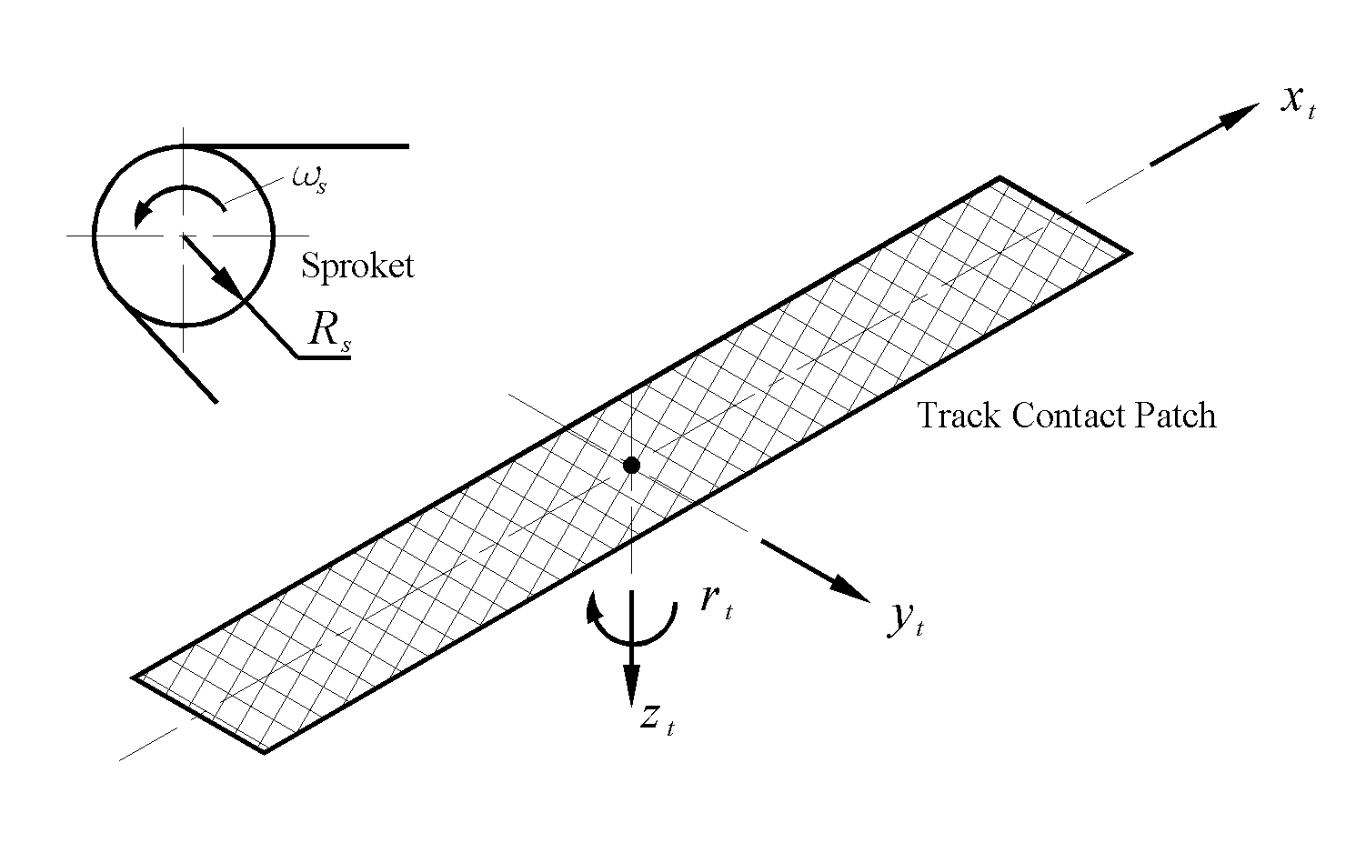
The axis system used for a single track is shown in Figure 1. The origin for the axes is at the plan centre of the contact patch and, when required, an additional subscript of l and r is added for the left and right tracks respectively. The angular speed of the sprocket is ωs and its radius is Rs.
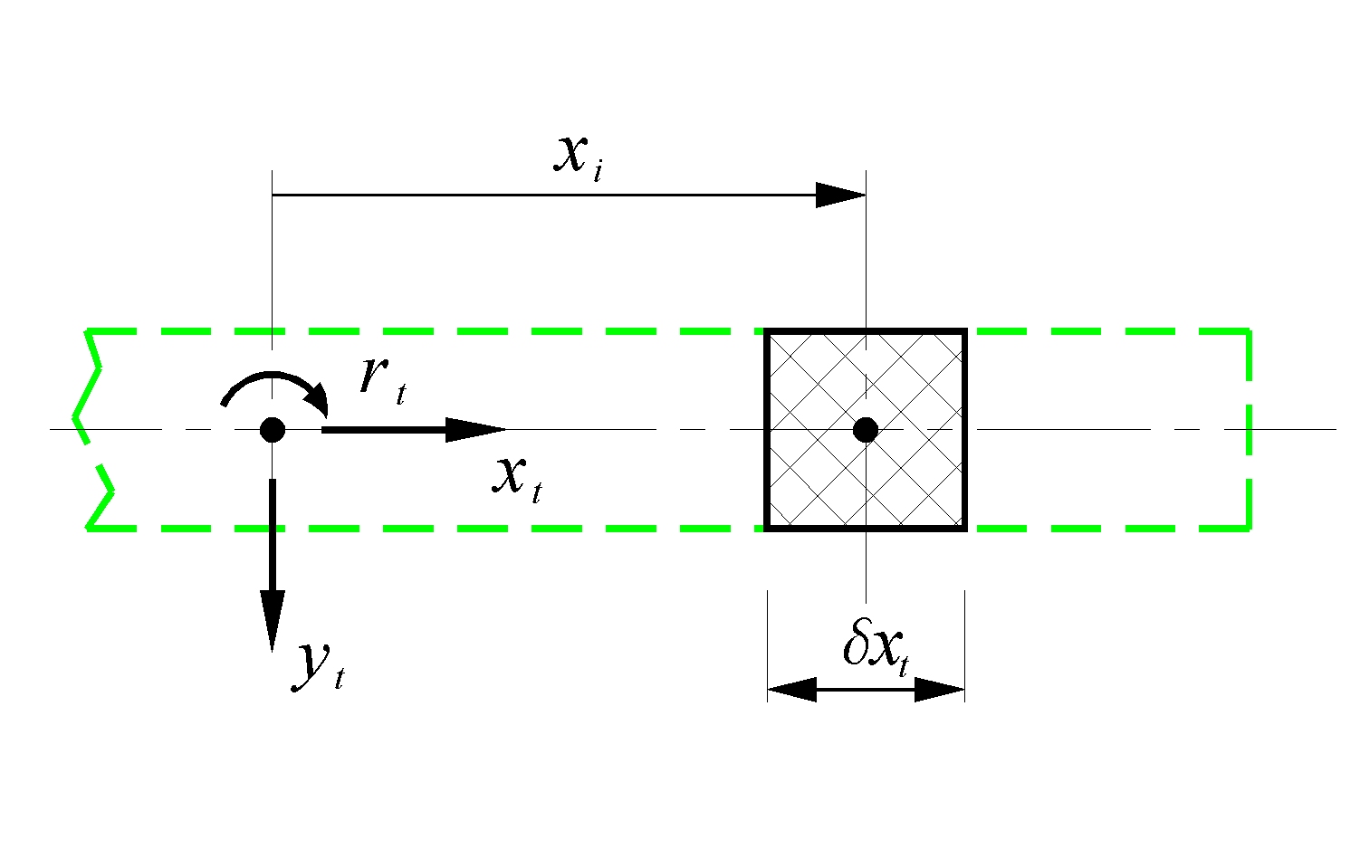
A plan view of the track is shown in Figure 2, in which the track has a forward and lateral velocities ut and vt, and yaw rate rt. A section of the track has been highlighted that is xi along the xt axis from the origin and is δxt long. From this diagram the longitudinal sliding velocity is given by:
(1)
which is the same all the way along the track. The sliding velocity in the yt direction at section i is:
(2)
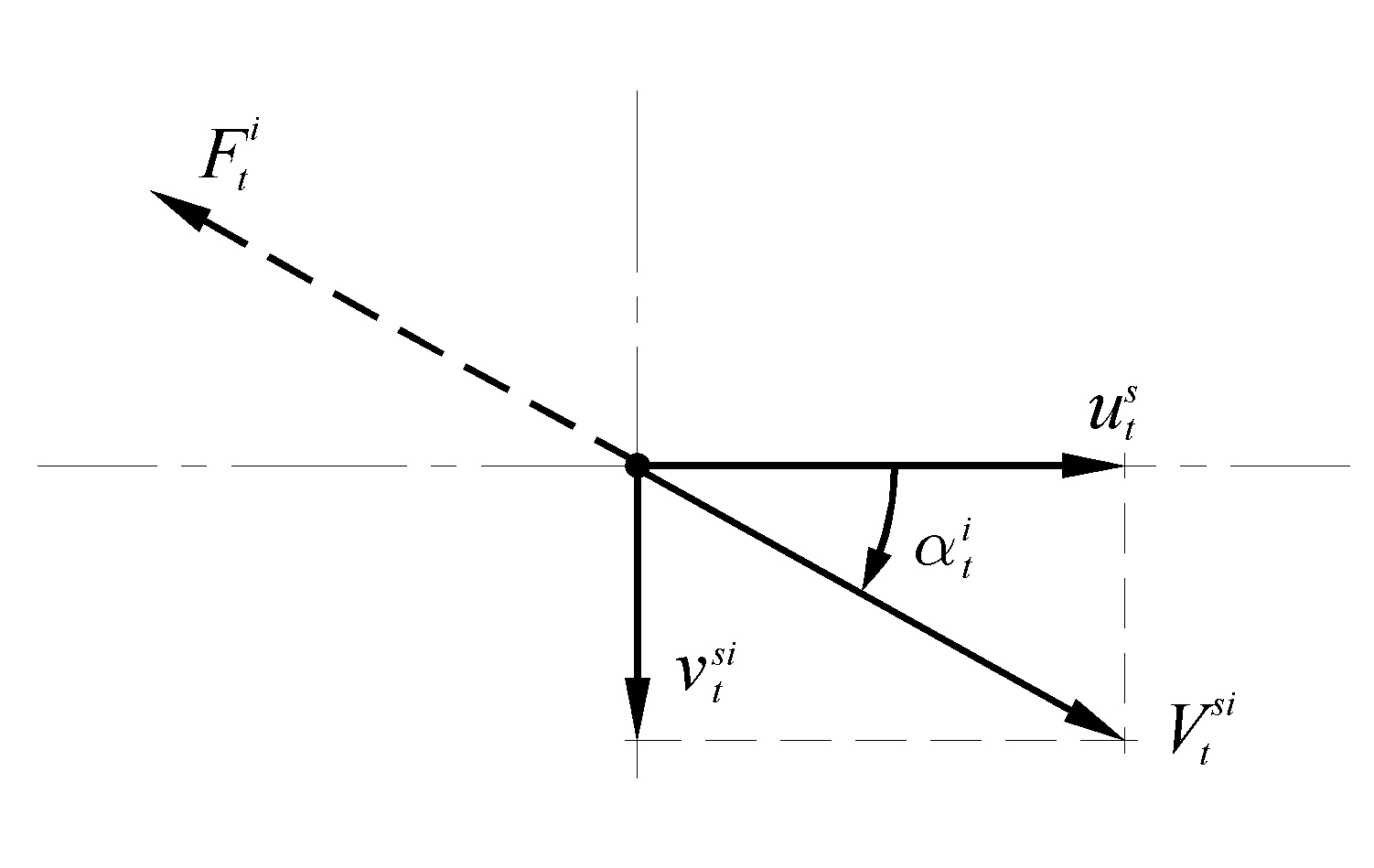
A diagram showing the sliding velocities of the track along the ground and the frictional forces, which oppose this motion at section i is shown in Figure 3. From this diagram the direction of motion of sliding and the velocity of the section are given by:
(3)
(4)
The longitudinal and lateral forces at section i are given by:
(5)
(6)
where the force opposing the sliding motion of the track is:
(7)
Thus the total longitudinal and lateral forces, and moment acting on the track by the ground can be derived. The longitudinal force is given by:
(8)
where the subscript i signifies that the summation is over the track. The lateral force by:
(9)
and the moment by:
(10)
Vehicle model
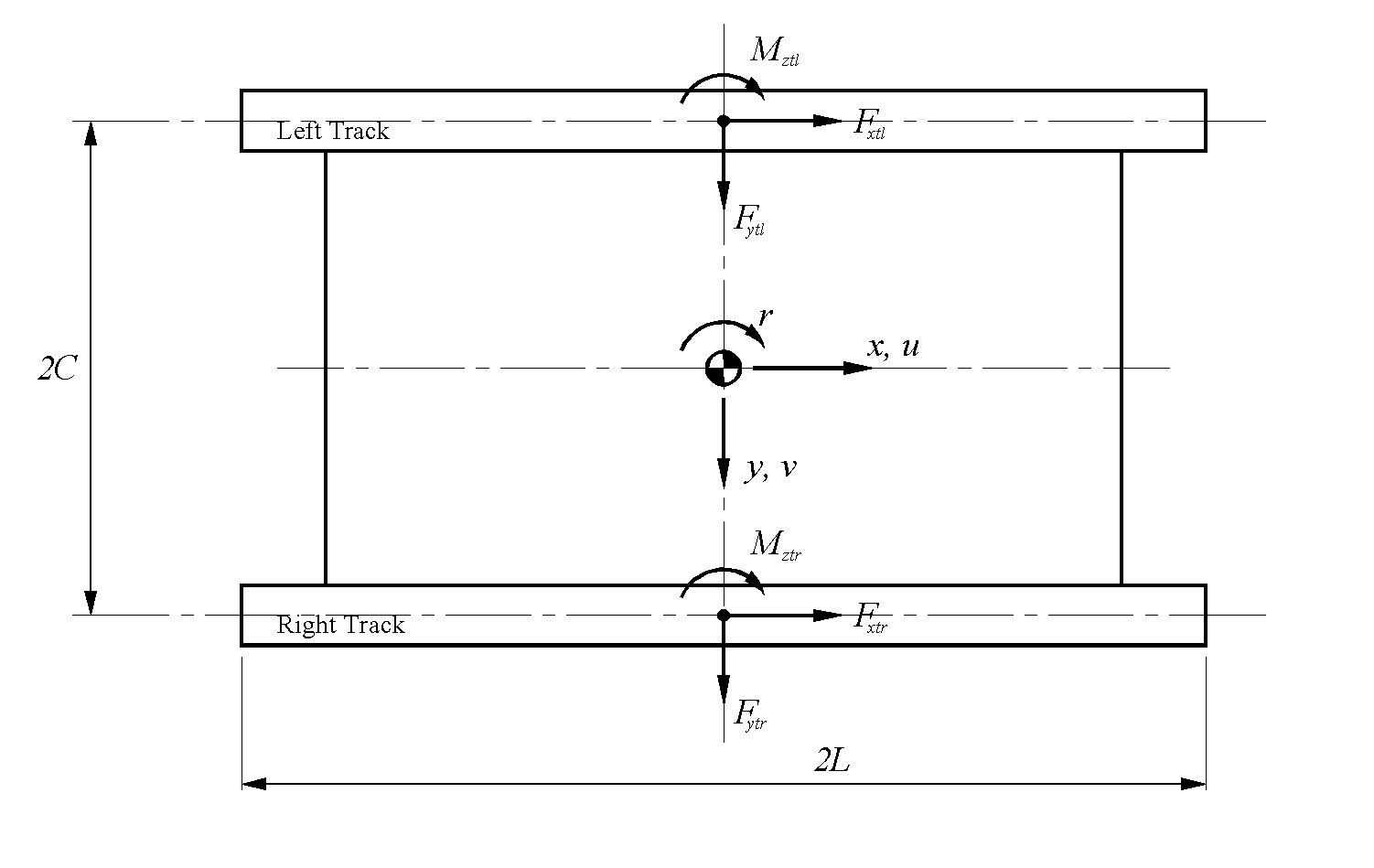
The vehicle model is developed using a body-centred axis system, which is commonly employed for vehicle dynamics. A free-body diagram of the vehicle is shown in Figure 4, in which the geometry of the vehicle is also defined.
The three equations of motion for the vehicle are:
(11)
(12)
(13)
where mv and Iz are the mass and yaw inertia of the vehicle. The first equation relates to the longitudinal motion of the vehicle, the second to the lateral motion and the third to the rotary (yaw) motion.
The weight transfer is incorporated into the model due to the centripetal acceleration. The free-body diagram of the vehicle turning to the right shown in Figure 5. From this diagram the vertical forces at the left and right tracks are given by:
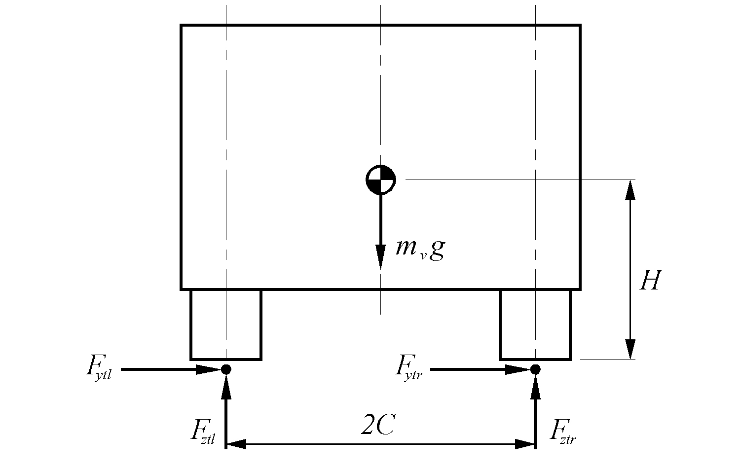
(14)
(15)
Experimental data
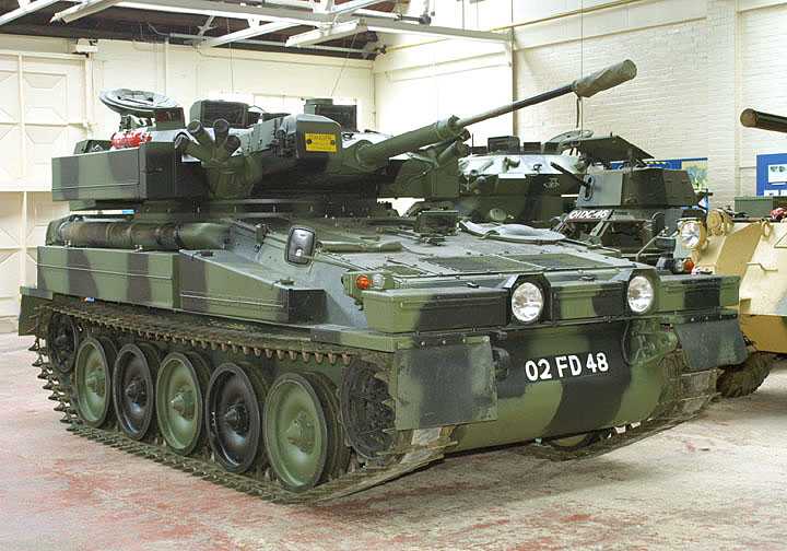
An experimental investigation into the handling characteristics of a lightweight tracked military vehicle has been undertaken in this study. The vehicle investigated was a CVR(T), which is based on Scorpion. A photograph of the vehicle is shown in Figure 6. The CVR(T) is part of a family of vehicles and in this configuration has five road wheels, the data for the vehicle is given in Table 1.
| Parameter | Value [Units] |
|---|---|
| Mass mv | 7938 [kg] |
| Yaw inertia Iz | 14 000 [kg/m2] |
| 2C | 1.716 [m] |
| 2L | 2.62 [m] |
| H (estimated) | 0.9 [m] |
The test consisted of driving the vehicle with a constant steer ratio n, at different speeds and measuring the lateral acceleration (latac) and radius of turn in steady state. Other parameters were also measured at this time but these are not discussed here. A plot of this data and a least-squares best-fit straight line for third gear is shown in Figure 7. The parameters for the best-fit straight line are; intercept R=5.22m and gradient 2.4 m/g (or 0.24 m/m/s2).
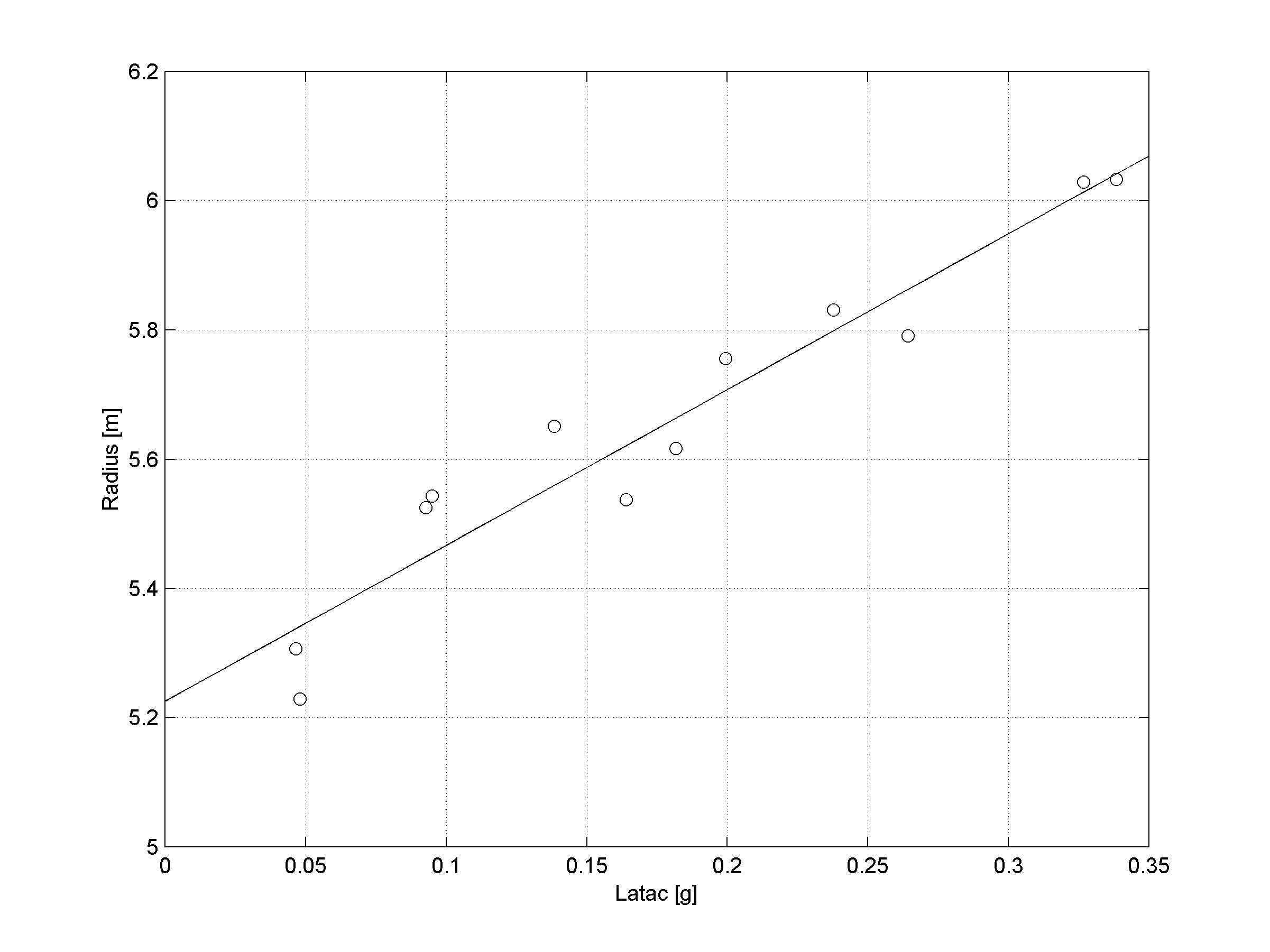
From Figure 7, the steer ratio at low speed/latac can be derived from [5] as:
(16)
where β is the non-dimensional slip radius. The slip radius is the instantaneous centre of sliding of the track on the ground and in this case is 0.37. From Equation (16), the low speed (latac) steer ratio is 1.69.
In this section the method used to simulate the motions of the CVR(T) are presented and the results of the simulation are discussed and compared with those from the experimental investigation.
The left and right sprocket angular speeds are given by:
(17)
(18)
where:
(19)
(20)
Simulation
In these equations the forward speed of the vehicle in straight running is Vn and the radius of the sprocket is Rs.
The transformation from the body-centre axis system to the earth based system is given by:
(21)
where ψ is the angle between the body and earth-based axis systems.
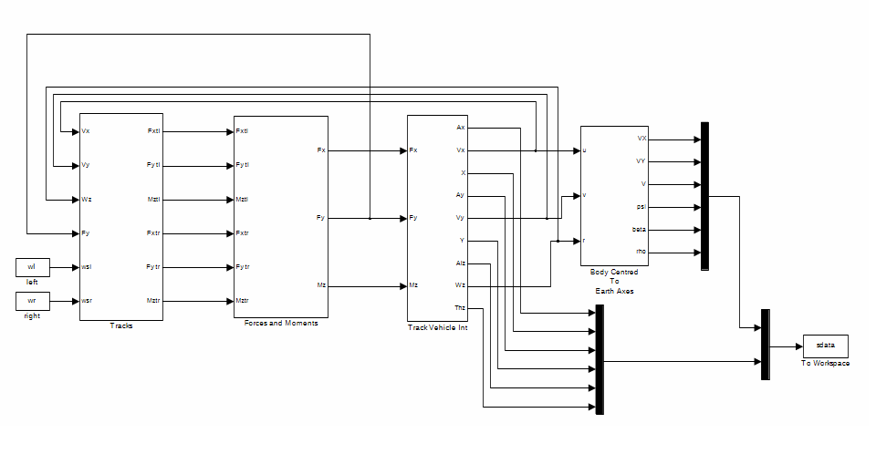
The equations given in the “Vehicle Model” section have been entered into Simulink [10], to allow them to be simulated. A block diagram showing the simulation model is shown in Figure 8.
Using simulation methods a study has been undertaken to investigate the variation of radius of turn with latac for a steer ratio of 1.69, as derived from the experimental data. A plot showing the results of this simulation for a coefficient of friction of 0.9 is shown in Figure 9. The value of coefficient of friction measured by for the CVR(T) track pad on the vehicle being investigated was 0.7 and the information given by Pott [9] for the possible track-ground sliding speeds to be encountered, indicates that this value would increase to approximately 0.9.
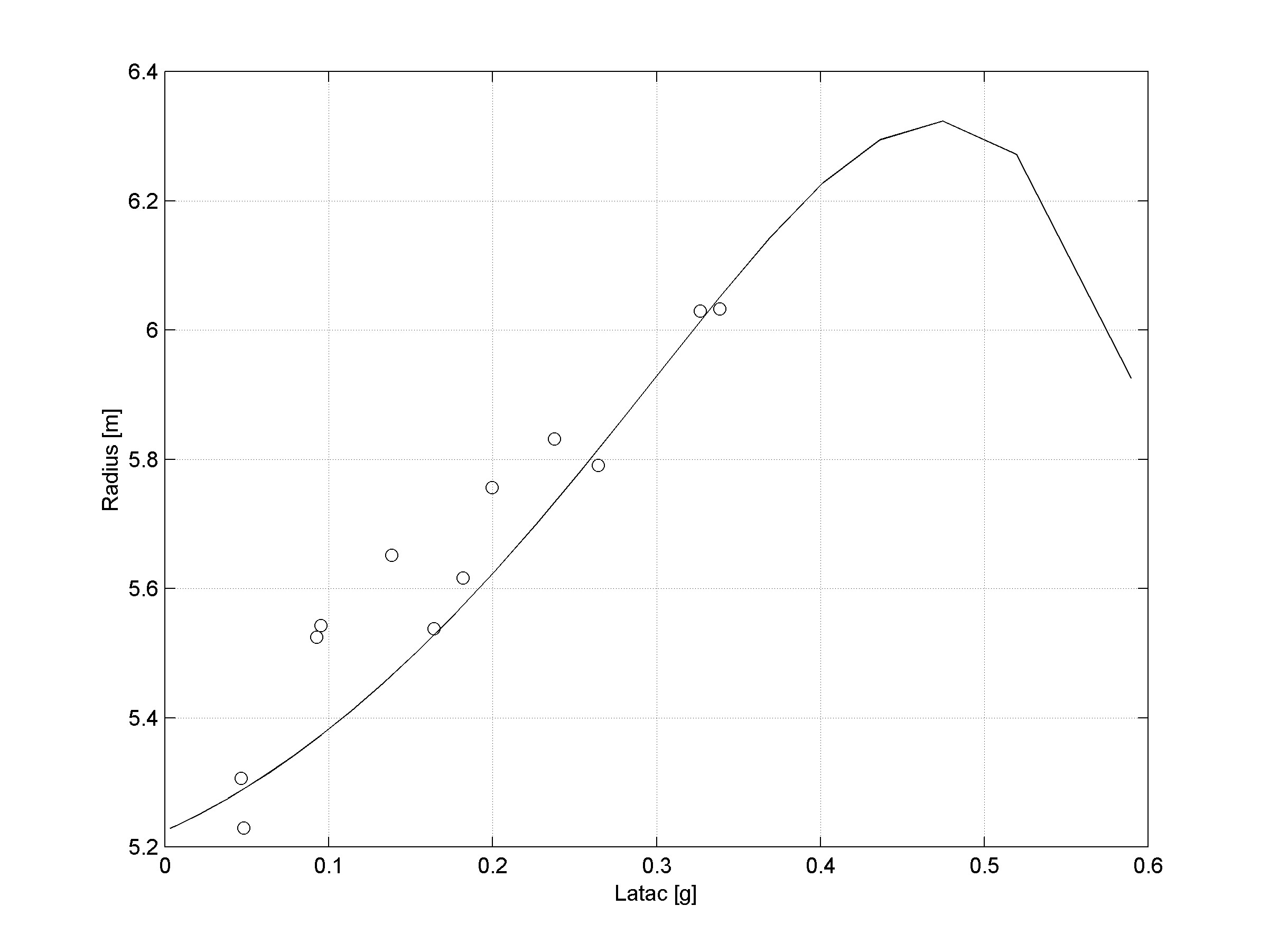
The data for Figure 9, has been obtained by running the simulation until the transient response has decayed and then examining the resulting radius of turn and latac. Two typical responses at low and high speed are shown in Figures 10 and 11.
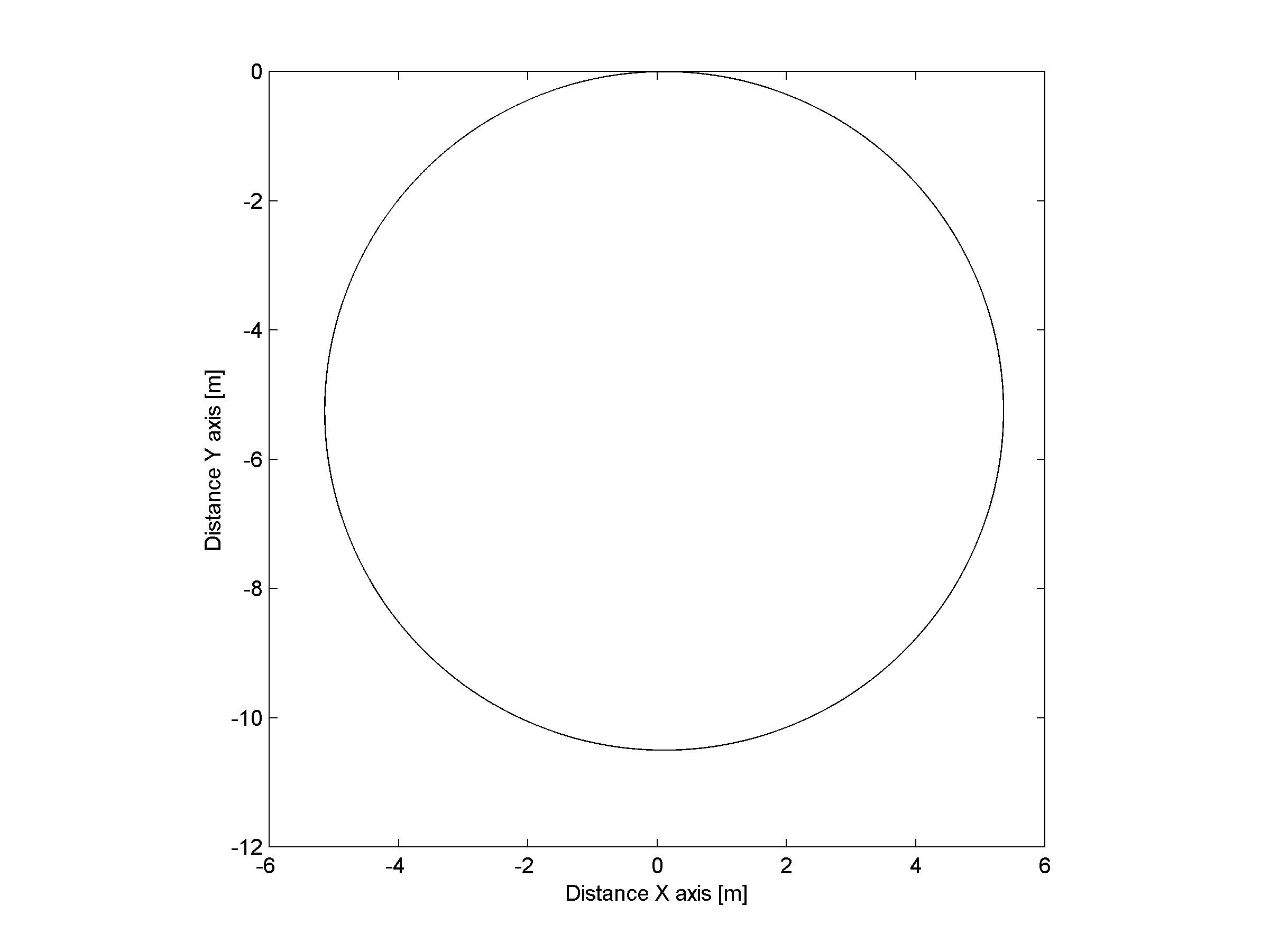
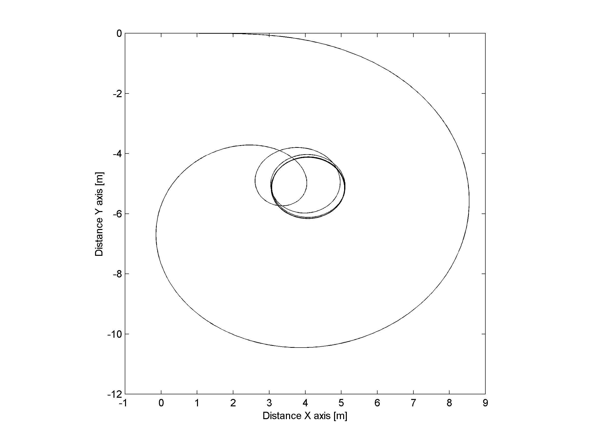
The simulation results shown in Figures 10 and 11, start at X=Y=0 and go clockwise. In Figure 10, the nominal speed of the vehicle is 1.0 m/s and the radius of turn is just over 5m with no visible transient. At 5.6 m/s, Figure 11, there is a considerable transient motion before the vehicle settles down to a radius of turn of about 1-m radius. These responses are typical of a tracked vehicle at different speeds [6].
The curve shown for the theoretical model with n=1.69, shown in Figure 9, has an initial increase up to latac of about 0.47g (4.6 m/s2) at a radius of approximately 6.3m. After the peak there is a rapid reduction in radius of turn with latac. This type of response is typical of a vehicle, which initially understeers and then goes into oversteer [11]. The experimental data has also been plotted on this figure and show a close correlation with the model.
To investigate the response of the vehicle further it is possible to use the model to predict the response of it for a constant radius turn, which is commonly used to investigate the handling of wheeled vehicles [11]. The results of a constant radius simulation are shown in Figure 12. This plot shows the steady-state steer ratio required to keep the vehicle on a 5.22-m radius. This type of test would be impossible to perform on CVR(T) because it has fixed steer ratios, which are dependent on the gear selected (1.69 in this case). It may be possible to carry out such a test on modern high-speed track layers (such as Alvis Warrior), which are equipped with continuously variable hydrostatic steering systems.
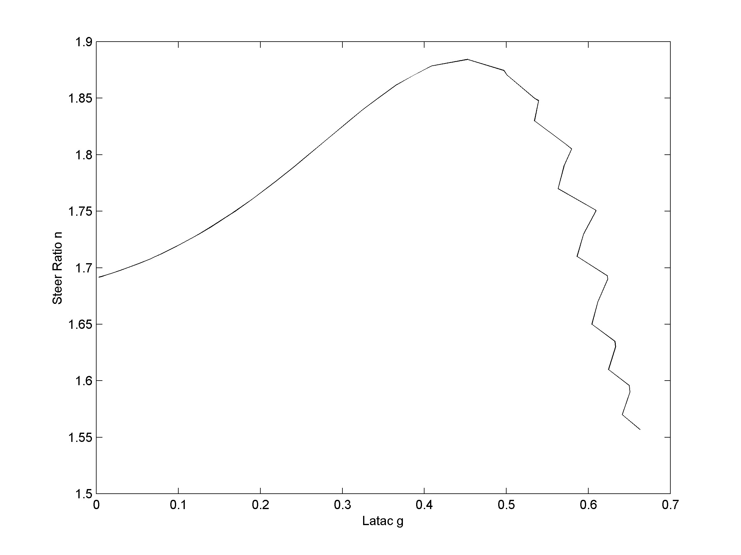
The results, of a simulation of a constant radius turn, at Figure 12, clearly show the transition from understeer to oversteer at 0.45g (4.4 m/s2). In the initial part of the plot an incremental increase in latac requires an incremental increase in steer ratio to remain on the required radius. At the peak, the response changes to one where an incremental increase in latac leads to incremental reduction in required steer ratio. The required steer ratio rapidly reduces at these higher latacs leading to terminal oversteer. In this final portion of the curve, control of the vehicle would become very difficult. Anecdotal evidence suggests that once the vehicle enters this region there is little that the driver can do to recover the situation. During the initial portion of the curve the required steer ratio changes from 1.69 to peak at 1.87, after which it rapidly falls to about 1.55. The initial understeer coefficient for the vehicle is about 0.5g.
Conclusion
In this study, a model of the steering characteristics of a tracked vehicle has been developed to include the effects of weight transfer due to lateral acceleration, using Simulink [10].
After validation, with test data from CVR(T) in fixed steer ration turns, the model was used to investigate the handling behaviour of the same vehicle in a constant radius turn. The simulations indicated that the vehicle would initially understeer before going into a limiting oversteer at 0.45g (4.4 m/s2).
References
[1] J. Wong, Theory of Ground Vehicles, John Wiley and Sons, 2001.
[2] T. Thai and T. Muro, “Numerical Analysis to Predict Turning Characteristics of Rigid Suspension Tracked Vehicles”, Journal of Terramechanics, Vol. 36, pp. 183-196, 1999.
[3] H. Merritt, “Some Considerations Influencing the Design of High-speed Track-Vehicles”, The Institution of Automobile Engineers, pp. 398-429, January 1939.
[4] W. Steeds, “Tracked Vehicles—An Analysis of the Factors Involved in Steering”, Automobile Engineer, pp. 143-148, April 1950.
[5] P. Wormell, Introduction to Skid Steering of Tracked Vehicles, MSc Handout, Royal Military College of Science.
[6] M. Kitano and M. Kuma, “An Analysis of Horizontal Plane Motion of Tracked Vehicles”, Journal of Terramechanics, Vol. 44, No. 4, pp. 211-225, 1977.
[7] J. Wong and C. Chiang, “A General Theory for Skid Steering of Tracked Vehicles on Firm Ground”, Proceedings of the Institution of Mechanical Engineers, Vol. 215, Part D, pp. 343-355.
[8] W. Ehlert, B. Hug, and I. Schmid, “Field Measurements and Analytical Models as a Basis of Test Stand Simulation of the Turning Resistance of Tracked Vehicles”, Journal of Terramechanics, Vol. 29, No. 1, pp. 57-69, 1992.
[9] S. Pott, “Friction Between Rubber Track Pads and Ground Surface With Regard to the Turning Resistance of Tracked Vehicles”, Proceedings 5th ISTVS Conference, Budapest, pp. 105-112, 1991.
[10] Matlab and Simulink, The MathWorks, Inc, Natick, MA, USA.
[11] J. Ellis, Vehicle Dynamics, London Business Books, 1969.