Weapon Scoring Using a Multilayer Perceptron Network

Introduction

Entering the new millennium does not guarantee us a safer world. Unfortunately, it is likely to project us toward a new era of defence and hostility in which we will see more destructive and more precise weapons. The defence industry is using technological advancement to produce various types of new and advanced weapon. Consequently, this will require continuous changes in the way weapon and force strengths are analysed. Weapon scoring has been used widely to determine the strength of combat forces with multiple weapon systems [1–3], with the aim of ensuring that an adequate defence structure can be established relative to the threat. Here we propose a new extendable method to determine weapon scores.

Problem statement

Weapon scores can be calculated using already developed formula. Kupchan [4] presented the formula used to calculate weapon scores referred as Weapon Effectiveness Indices (WEI). The generic equation used for a weapon is:

$WEI=C_{f}F+C_{m}M+C_{s}S$

where:

F = firepower index for the weapon;

M = mobility index for the weapon;

S = survivability index for the weapon; and

C_{(f, m, and s)} = weighting coefficients for the category.

The effectiveness coefficients were determined by military judgement. In the case of tanks, the indices are calculated through the following equations:

$Firepower,F=C_{a}ADC\times P+C_{f2}FM+C_{n}N+C_{a2}AF$$+C_{w}W+C_{c}Com$$Mobility,M=C_{g}GP+C_{c}2CR+C_{g}2GC+C_{v}V+C_{s}2SL$$+C_{t}T+C_{w}2WO+C_{r}RS+C_{g3}GW+C_{l}LVE$$+C_{t}2TC+C_{l2}LWT$$Survivability,S=C_{a2}AP+C_{p}PA+C_{h}H/T+C_{a3}AS+C_{a4}AD$$+C_{\text{f3}}\text{FE}+C_n\text{NBC}+C_{\text{f4}}\text{FS}$ + CrRS + Cg3GW +

where:

ADC = armour defeating capability

P = stabilisation factor

FM = fire mission time

N = limited visibility

AF = ammunition types available and basic load

W = auxiliary weapons available

Com = intercommunications

GP = ground pressure

CR = cruising range

GC = ground clearance

V = step vertical obstacle traversing

SL = slope climbing

T = trench spanning

WO = water obstacle crossing

All C’s with subscript are weighting coefficients

RS = road speed

GW = gross weight

LVE = limited visibility enhancement

TC = vehicle commander to driver intercom

LWT = length/ width track pad

AP = armour protection

PA = presented area

H/T = horsepower/ ton

AS = ammunition storage

AD = active defensive systems

FE = fire extinguishing systems

NBC = nuclear, biological, chemical defence systems

FS = fuel storage.

As we can see, determining all the weighting coefficients is very crucial. Furthermore, obtaining comprehensive and accurate weapon data is critical but difficult, especially from non-allied countries or a biased weapon industry. Therefore, the problem with the previous procedure is that some of the required data might be missing or misleading. To overcome the problem, we have developed a neural network method to determine the weapon score using whatever data are available. As some of the physical data of weapons are correlated, we presume a trained MLP network is capable of negotiating missing and misleading data and will provide the best possible score relative to the training data used. To train the MLP network, we use weapons with scores calculated from WEI [5]. However, we also use more weapon criteria, and the network will generate the appropriate weight toward each criterion. Therefore, we obtain a more generalised way to determine weapon scores.

Implementation

Input layer—weapon data

Weapon systems are divided into two main components comprising of a weapon platform and the weapon systems. Each weapon platform might carry more than one weapon. Therefore, for each weapon system, data are collected are as shown in Table 1. There are fifteen data items required for each weapon platform and thirteen data items required for each weapon. However, categorical or non-numerical data, such as weapon group (small arms, artillery, tank, APC, aircraft, and so on) and type of guidance system (optical, laser-guided, and so on), will be broken down into choices and treated as binary data. For example, input for the optical guidance system for a weapon will be ‘1’ for yes, if it is optically guided, or ‘0’ otherwise. Therefore, the number of inputs required will be 28 for each weapon platform and 17 for each weapon system. Assuming a maximum of four weapons types for a weapon system, therefore, for each weapon system, the maximum number of inputs required is 96 (that is 28 + 4x17). This determines the size of the Input Layer, which will be equal to the number of inputs. The data can range from zero to infinity with different units of measurement. However, before the data is used to train the network, the data is scaled to within -1 and 1 so that they always fall within the specified range. This pre-processing step for the network input is required to make the neural network training more efficient [6].

Output layer—weapon score and mapping factor

The output layer consists of nine neurons. The main output is the weapon score. This weapon score will measure effectiveness of a weapon within its category. It can take any positive value. However in our analysis we will scale it down to 0 to 1. This is done to make the weapon score output on the same scale with the other 8 outputs that are within 0 and 1. Therefore, we can use same transfer function (as discussed later) for all outputs; thus our network is simpler. The higher the weapon scores the better the weapon within its category. The other eight outputs are the Mapping Factors (MF) for each force element strength as shown on Figure 1. As stated, the MF can take any value from 0 to 1 for each element. The Mapping Factor reflects the degree of contribution each weapon can provide towards individual element strengths. A zero value means the weapon cannot contribute any strength towards that element while the value of one reflect that the weapon can contribute its full strength towards the element. All other values in-between reflect the degree of contribution the weapon can provide towards the strength of each element.

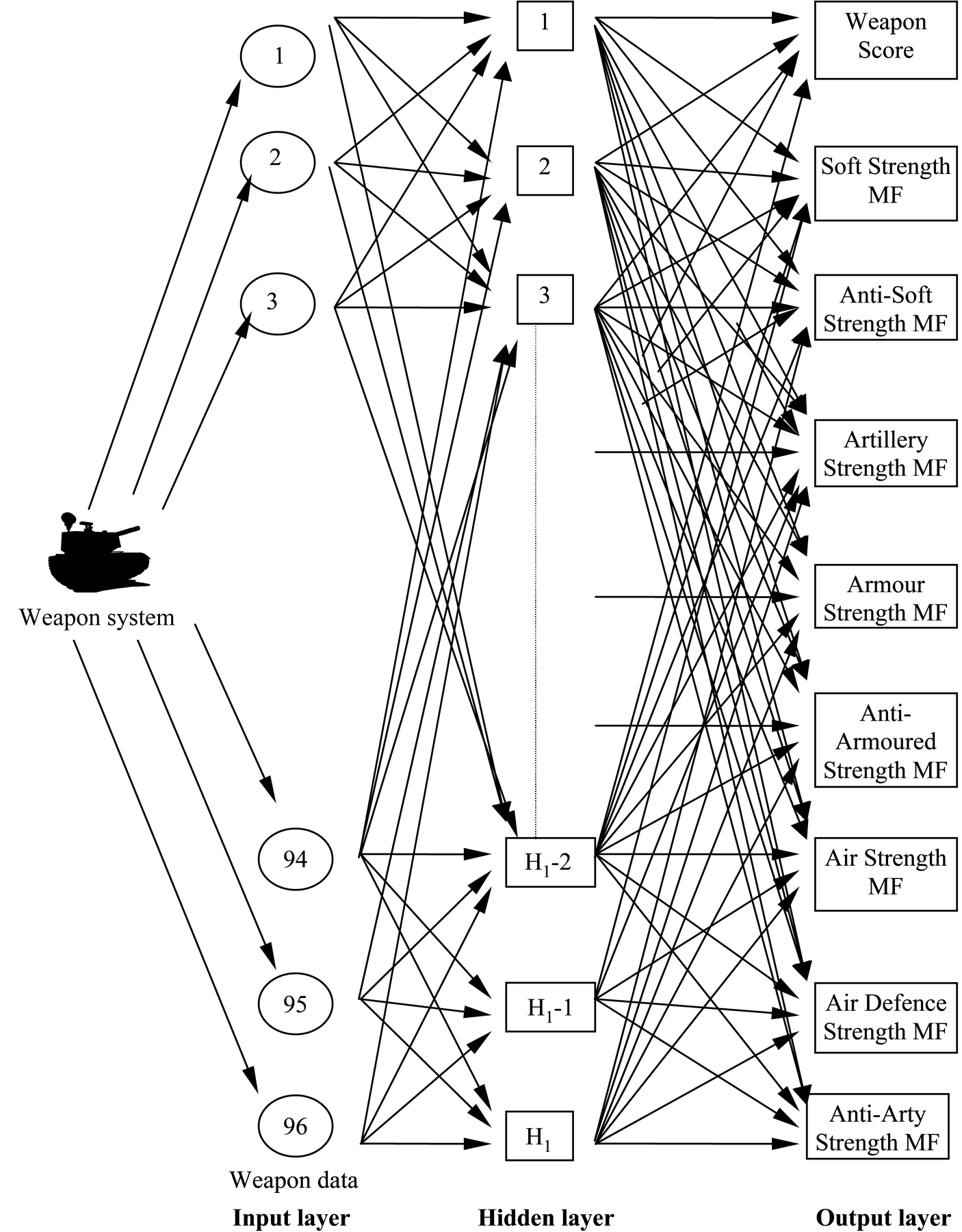
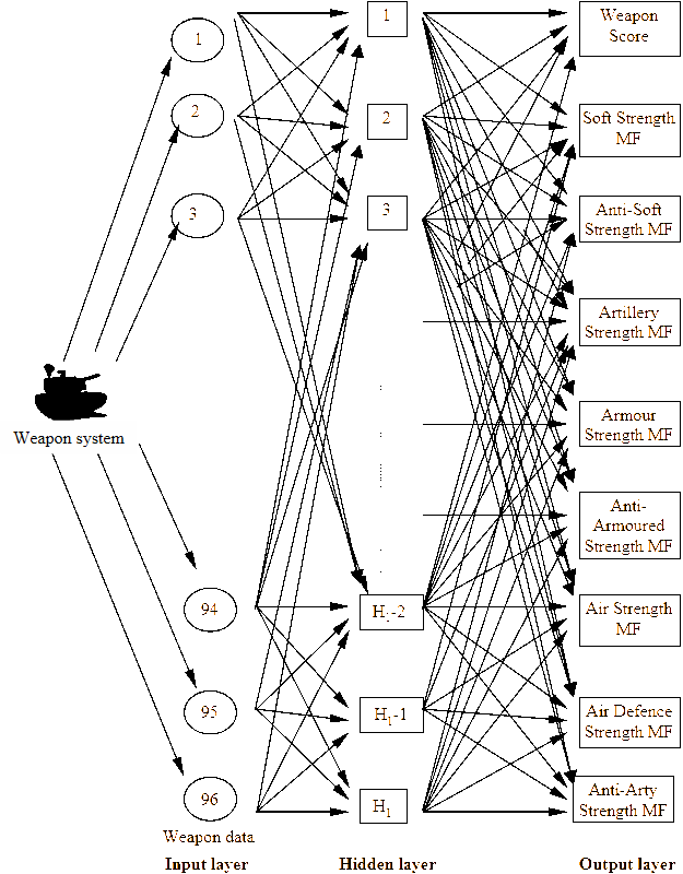
Multilayer perceptron network

The artificial neurons in the hidden and output layers process values received from neurons in the input layers. A processing neuron multiplies each input value, x_i, from neuron i, by scalar weight, w_i, representing the strength of the connection, as shown in Figure 2. The combined input sum x_iw_i and bias, b, is then input to a transfer function that determines the activation level, a, of the processing neuron. Since all the output is expected to fall within 0 and 1, all the transfer functions used for output layer are binary sigmoid or log sigmoid. Thus, by using the log sigmoid transfer function, the values of 'n' that can take any value, will be transferred using the transfer function into values of 'a' that will be within 0 and 1.

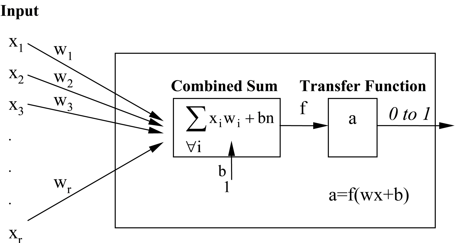
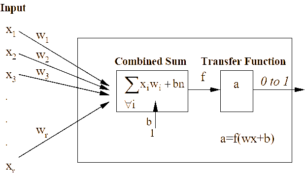
Sampling and training

A total of 65 weapon data of various categories were gathered for the initial process of training, validation and testing. Out of the 65, one third was saved for testing and another one-third for validation. The remaining weapon data (21) was used for training. The number of training samples seems very low compared to the number of weights and biases to be trained. The validation sample set is used for the early stopping procedure, which will be discussed later. For other methods this validation set will be used for training together with the training samples. The test data will be used to test the performance of the trained network to ensure that their outputs will be within the relative targets.

Mehrota et. al. [10] pointed out the complexity of ways to determine size of training samples or size of the network. They stated that, in practice, specific problems are solved using trial and error. However, they suggested a rule of thumb, obtained from related statistical problems, is to have at least five to ten times as many training samples as the number of weights to be trained. While, Baum and Haussler [11] suggest the following number:

$P>\frac{\left|W\right|}{1-a}$

Where P denotes the number of patterns (i.e., the size of the training set), |W| denotes the number of weights to be trained, and a denotes the expected accuracy on the test set. Thus, if our 96-30-9 network contains 3150 (96x30 + 30x9) weights and the desired test set accuracy is 90% (a = 0.90), then their analysis suggests that the size of the training set should be at least, P > 3150/0.10 = 31500. Unfortunately, for our problem it will not be very practical to obtain such a huge sample. Thus, we performed the test using samples available at hand and the results (presented next) are very encouraging.

Testing and analysis

We implemented the problem in MATLAB with the Neural Network toolbox. We tried several training algorithms to get the global optimum weight and biases [6]. The Levenberg-Marquardt algorithm and the BFGS Quasi-Newton algorithm require too much memory, therefore they did not work well. Also, the Bayesian Regularisation technique takes a long time to solve this problem, in addition to requiring a large amount of computer memory. Our attempts using Scaled Conjugate Gradient algorithm seem to be working reasonably well, but we still have a problem with local optimum. We have to run the algorithm several times to ensure we achieve either the global optimum result or something close to it.

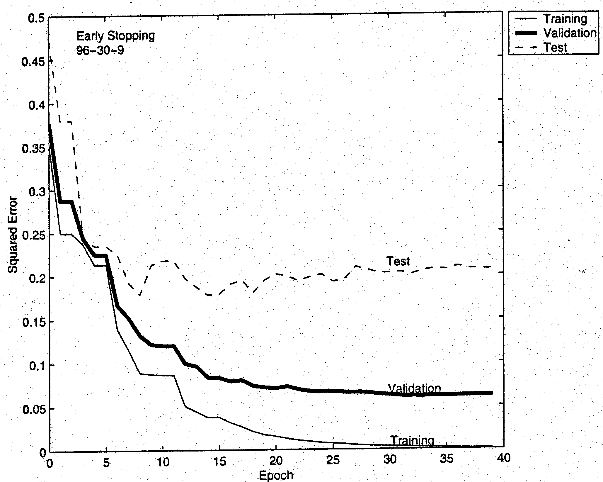
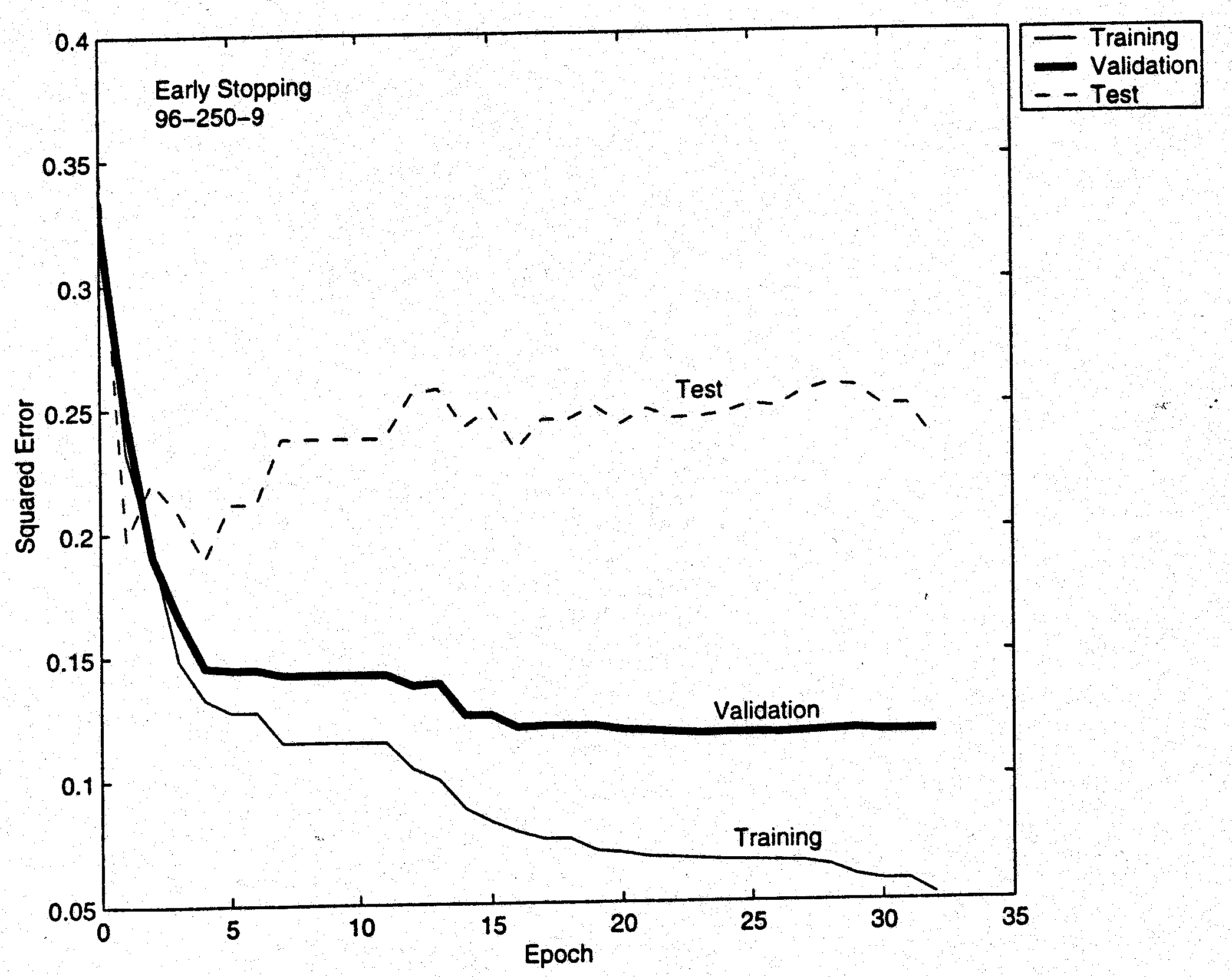
Early stopping is a method use to improve generalisation. It is a good alternative approach for nets with small number of training cases compared to parameters. It is fast and can be applied successfully to networks in which the number of weights far exceeds the sample size. It needs a large number of hidden units, very small random initial values and a slow learning rate [8]. In implementing this technique, we use the three subsets of data. The training set is used for computing the gradient and updating the network weights and biases. The second subset is the validation set. The validation set can be regarded as a bias test set to check on errors in every iteration. Thus, the error on the validation set is monitored during the training process. The errors for both subsets will normally decrease during the initial phase of training. Then the network begins to overfit (or ‘overtrain’) the data, meaning that the error for the training set continue to decrease whilst the validation set error begins to rise. Thus, after the validation error increases for a specified number of iterations, the training is stopped, and the weights and biases at the minimum of the validation error are returned. The third subset is the test set. It is not used during the training, it is used as an unbiased estimate of the generalisation performance. It can and will also be used to compare different models. If the error in the test set reaches a minimum at a significantly different iteration number than the validation set error, this may indicate a poor division of the data set [6].

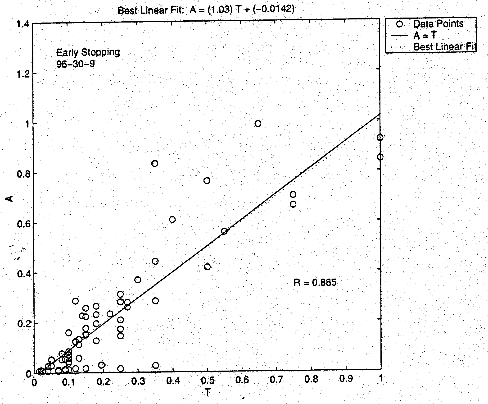
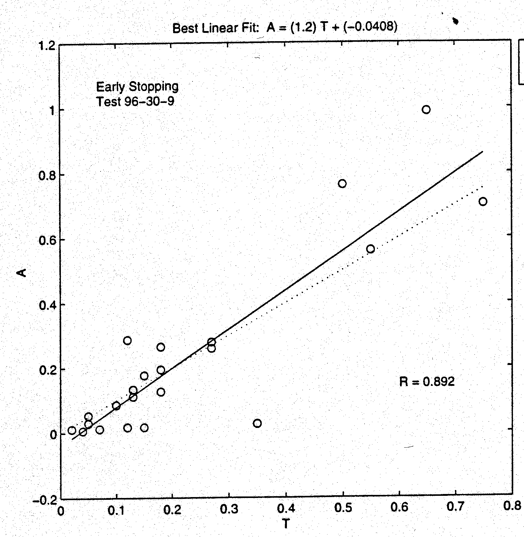
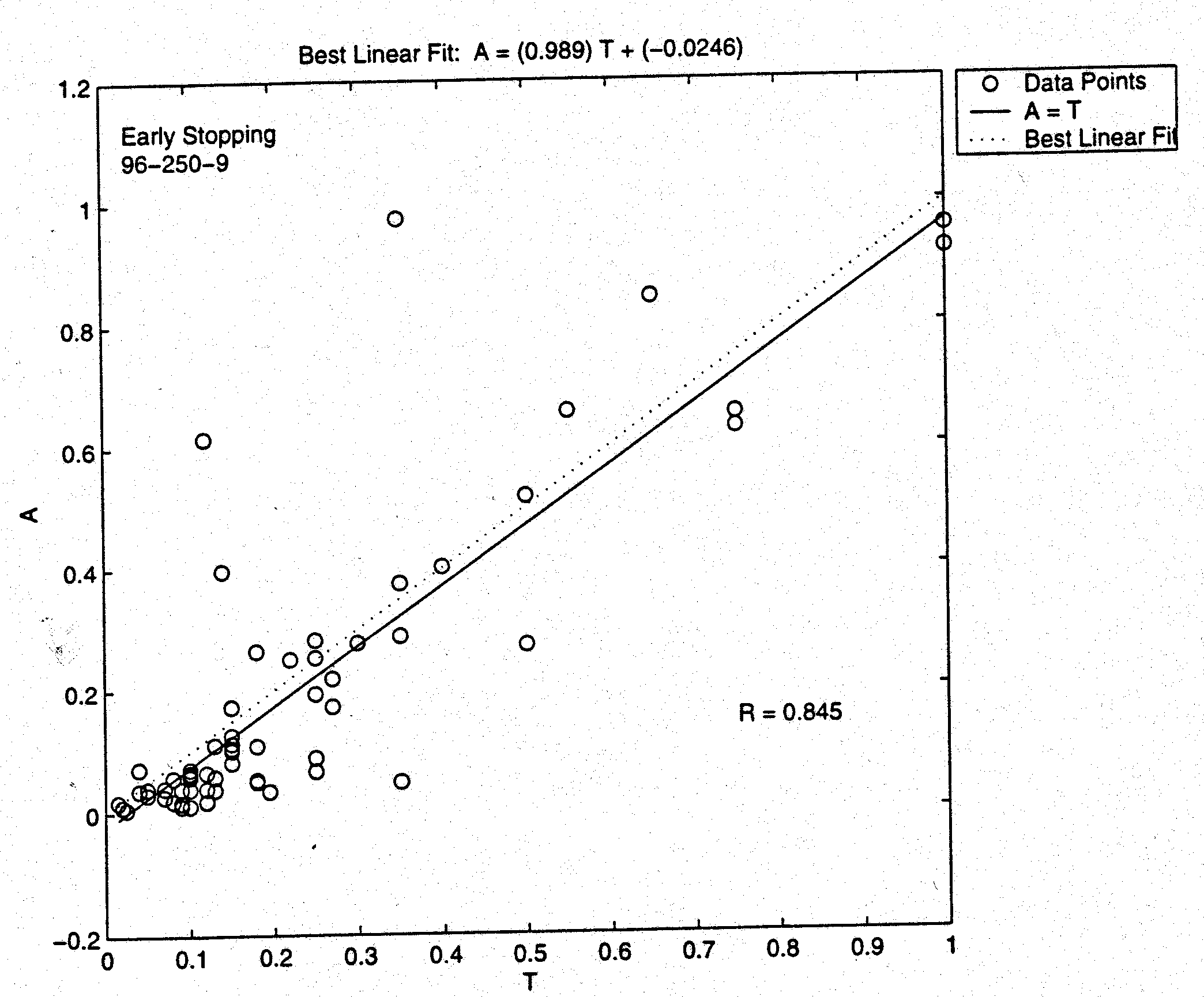
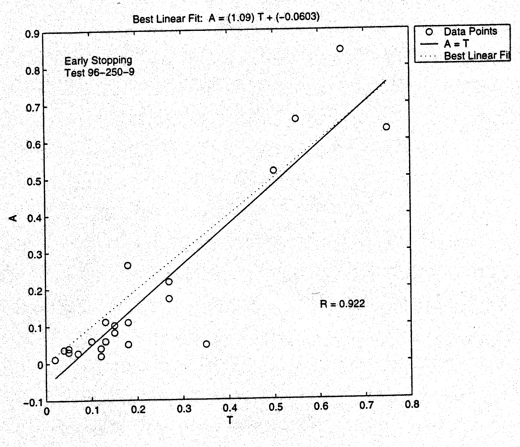
The resulting analysis is performed using linear regression between the network outputs and the corresponding target. The ideal result would have the 'A=T' line fall on top of best linear fit line, meaning the slope (gradient), m, is one and the interception at the Y-axis, c, is zero, or A = (1.00)T ± 0.00, whilst the correlation, R-value, equal to 1. The performances using early stopping technique are shown on Figure 3 to Figure 8. Figure 3 to Figure 5 show results for 30 hidden units network architecture, and Figure 6 to Figure 8 show results for 250 hidden units network architecture. As stated earlier, network with large numbers of hidden units with 250 hidden units provides better results with R = 0.922, m = 1.09, and c = -0.06, as we can see on Figure 8. Whilst with only 30 hidden units the result as can be seen on Figure 5 are R = 0.892, m = 1.2, and c = -0.04. However, for both architectures, 96-30-9 and 96-250-9, we can see in Figure 3 and Figure 6 that the error for the test set is quite high compared to the validation set. Furthermore, the error in the test set reaches a minimum at a significantly different iteration number than the validation set error. Therefore, our next step is to present analysis using set goal performance rather than early stopping. Set goal performance means we will set the level of error as a goal to be achieved; once the training reached the set level of error the iteration will stopped, then the network will be tested.

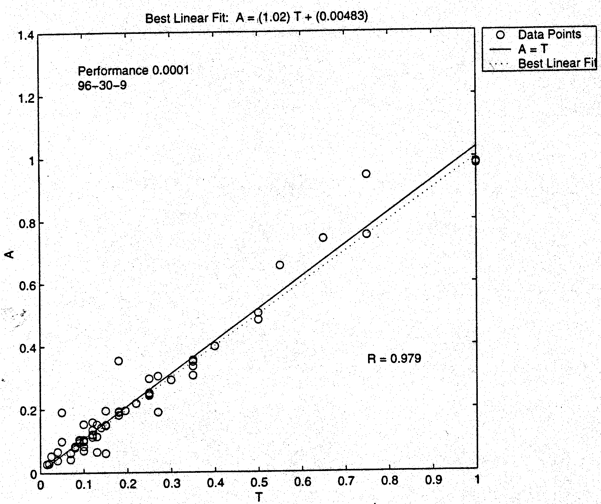
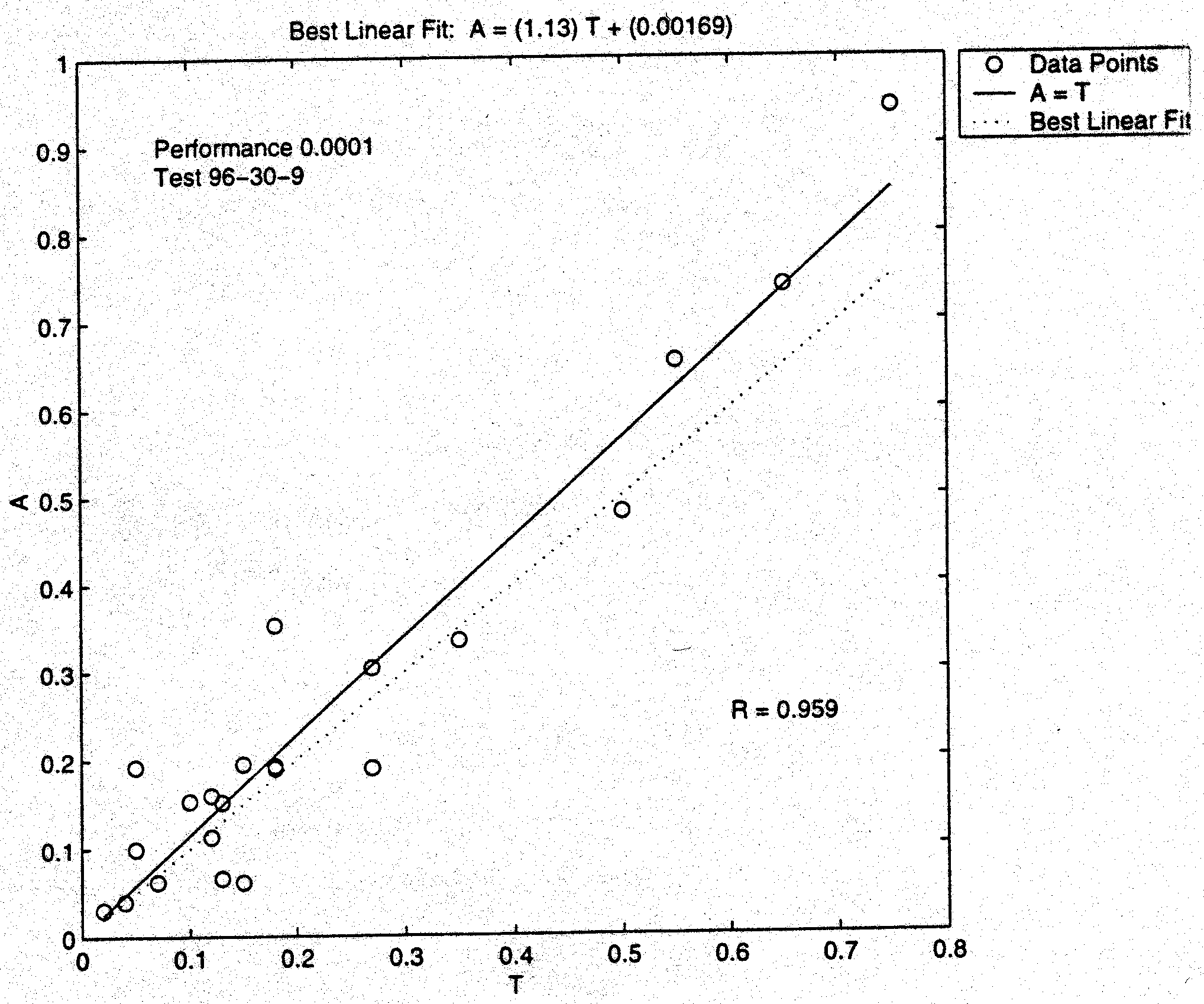
Since we are not using the early stopping technique we will focus to the network that gives the best result, with the lowest number of hidden units. Figure 9 and Figure 10 show us the same regression for the same network architecture as Figure 4 and Figure 5 but using target error instead of early stopping. The target error is set at 0.0001 and reached after 137 iterations. We can see on the regression figures, the main output for all data sets seem to track the targets reasonably well, better than the one from early stopping, and the R-values are more than 0.95. Thus our finding for this case was that the result using the network architecture of 96-30-9 performed the best. The final result using the chosen architecture is good since even the test set performs reasonably well as shown on Figure 10.

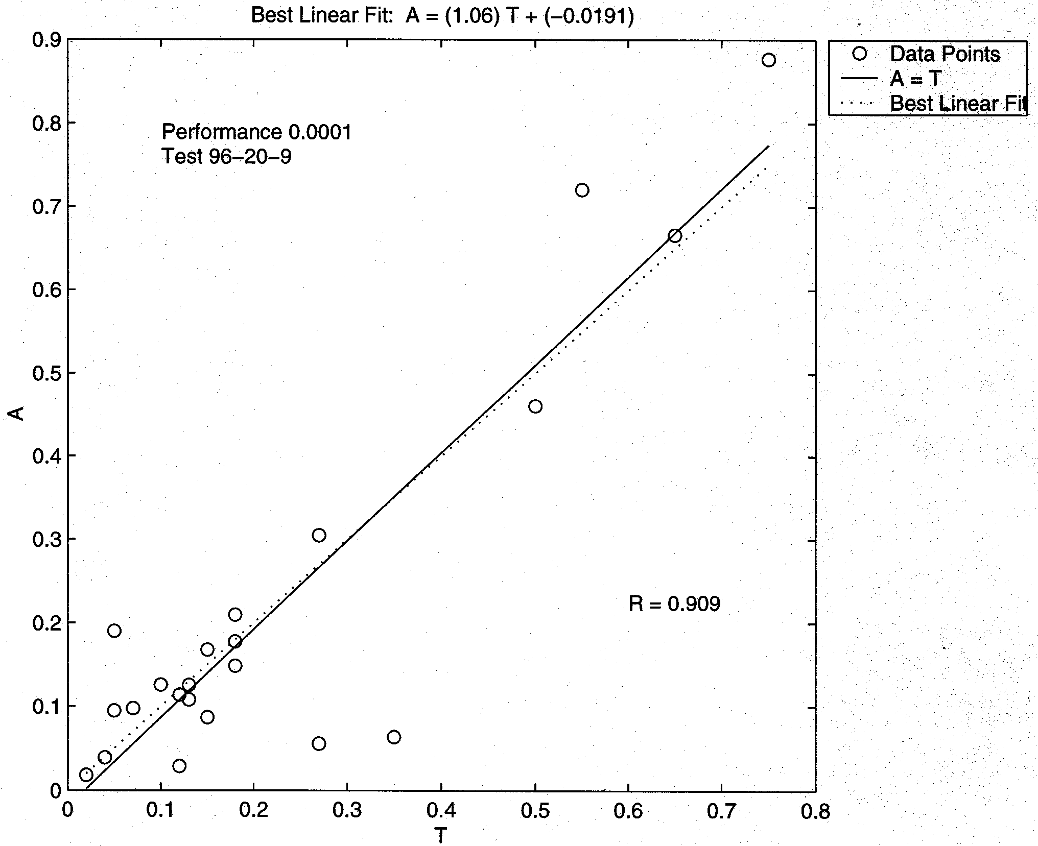
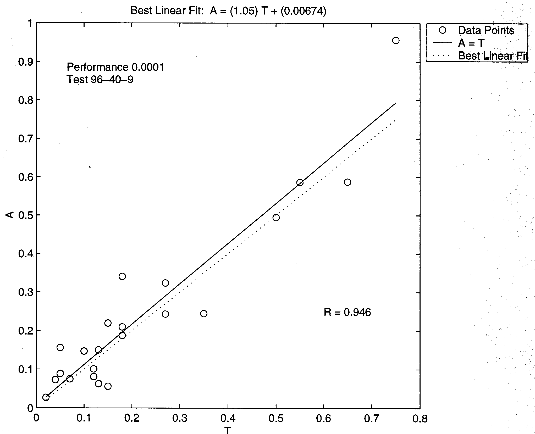
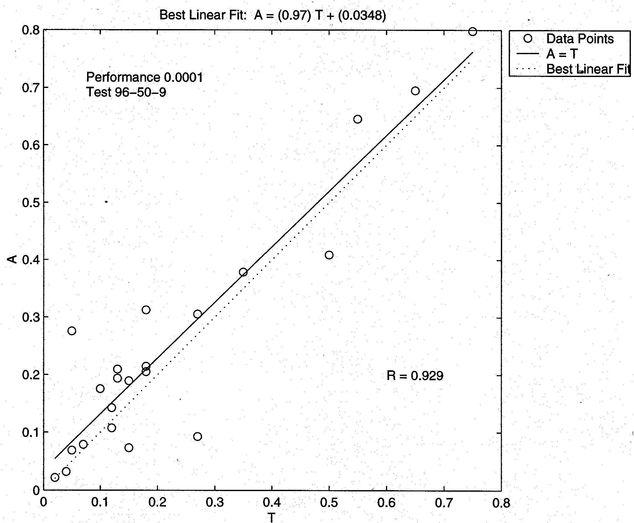
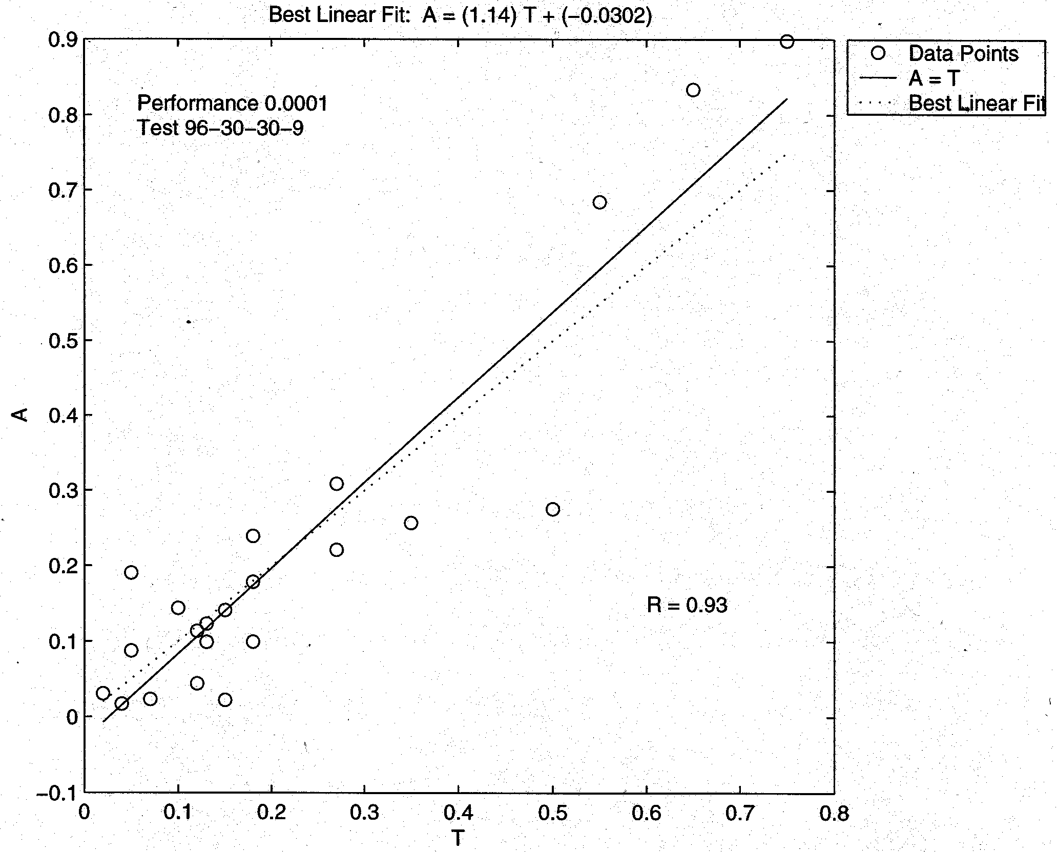
For comparison we also tried other network architectures. Other architectures with smaller or larger hidden units will not improve the performance anymore (Figures 11 to 13 ). While a two hidden layer network will not make the network any better (Figure 14). For the network 96-30-9 all other outputs (that is, the mapping factor, MF), we can see that the best linear fit and the perfect fit line (A = T) are very close. R- values and the slope seem to be very close to 1, and the y-axis interception is close to zero. Two of them are as shown in Figure 15 and Figure 16.

Conclusion and further work

Backpropagation can train multilayer feed-forward networks with differentiable transfer functions to perform weapon scoring. The result shows that the small sample used does not mean we cannot get a reasonably good generalisation from the training. The architecture of a multilayer network is not completely constrained by the problem to be solved. Except for the number of input and output neurons which are determined by the problem, the number of layers between them and their sizes are up to the designer.

For further work it would be good to pursue more samples for training, and validation. Further investigations with a more powerful machine should be done to search for the best algorithm to generalise the network. By doing so, we will be able to generalise better and increase the credibility of weapon scoring.

Acknowledgement

This research is sponsored by the Malaysian Armed Forces.

References

Authors

Maj Norazman B M Nor is an officer in the Royal Engineer Corp, Malaysian Army. He is a Corporate Member of the Institute of Engineer Malaysia, and is currently pursuing PhD in Military Operational Research from the Royal Military College of Science, Cranfield University, Shrivenham, UK.

Dr Kathryn Wand is with the Applied Mathematics & Operations Research Group, at the Royal Military College of Science, Cranfield University. Her current research interests include the comparison of combat models, the modeling of military logistics and the incorporation of command and control into Lanchester type models.

References

[1] J. Epstein, Conventional Force Reductions: A Dynamic Assessment, The Brookings Institution, Washington DC, 1990.
[2] J. Bradford, “Quantitative Modelling of Modern Land Warfare: Operation Desert Sword (1991)”, Defence Analysis, Vol. 14, No. 3, pp. 277-298, 1998.
[3] T. Dupuy, Numbers, Predictions and War, Hero Books, Fairfax, Virginia, 1985.
[4] C. Kupchan, “Setting Conventional Force Requirements: Roughly Right or Precisely Wrong?” World Politics, Vol. 41, No. 4, pp. 536-578, 1989.
[5] P. Allen, Situational Force Scoring: Accounting for Combined Arms Effects in Aggregate Combat Models, Rand-Note, RAND, Santa Monica, 1992.
[6] H. Demuth and M. Beale, Neural Network Toolbox: For Use With MATLAB, User Guide Version 3, The MathWorks, Inc., MA, USA, 1998.
[7] M. Vaughn, “Interpretation and Knowledge Discovery from the Multilayer Perceptron Network: Opening the Black Box”, Neural Computing & Application, Vol. 4, pp. 72-82, 1996.
[8] W. Sarle, Neural Network FAQ, http://www-leibniz.imag.fr/RESEAUX/osorio/faqs/FAQ.html. Last modified: 16 May 1997.
[9] L. Fausett, Fundamentals of Neural Networks: Architectures, Algorithms, and Applications, Prentice Hall, New Jersey, USA, 1994.
[10] K. Mehrota, C. Mohan, and S. Ranka, Elements of Artificial Neural Networks, MIT Press, Massachusetts, 1997.
[11] E. Baum and D. Haussler, “What Size Net Gives Valid Generalisation?”, Neural Computation, Vol. 1, pp. 151-160, 1989.